
深度学习的反向传播笔记
深度学习反向学习方法可以说是神经网络中比较难懂的一块了,主要是公式的推导和计算要有一些数学知识
可以说这个思想的精髓是数学也不为过
因为都是数学公式表达式,不知道怎么发,直接转成了图片,可以放大查


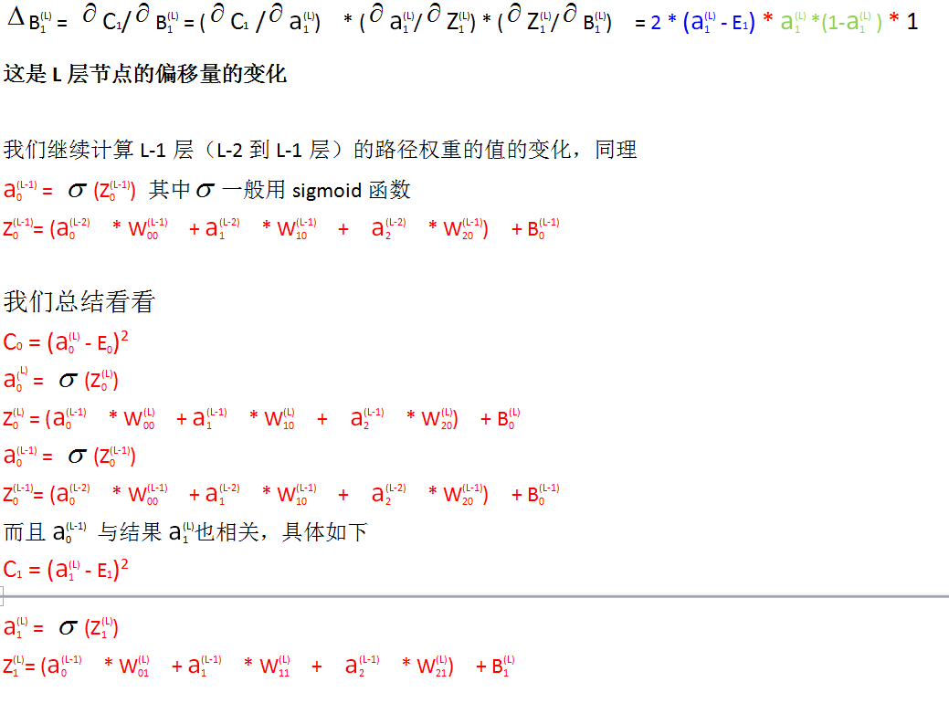
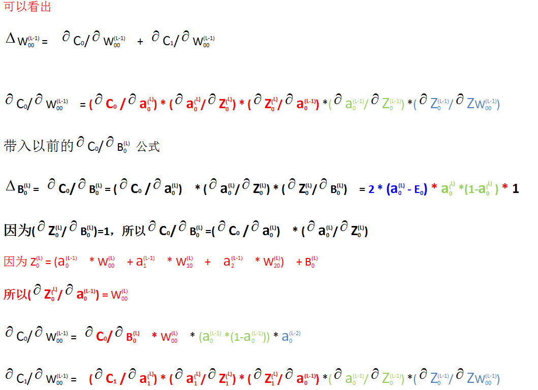
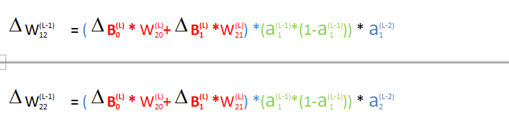
这里的误差推荐用平方差


每次学习神经网络,看到反向传播都有点蒙,做个标件,以后如果还有什么再补充~~~
2019年9月24号修正
 1 backprop(Dwtab, Dbtab, Tlist, Val, N) ->
 2     {_, Tname} = lists:keyfind(N-1, 1, Tlist),
 3     V = ets:tab2list(Tname),
 4     {_, Ntname} = lists:keyfind(N, 1, Tlist),
 5     ok = do_work2(Dwtab, Dbtab, Ntname, N, Val, lists:nth(N, ?NETWORK), V),
 6     backprop(Dwtab, Dbtab, Tlist, N-1).
 7
 8 do_work2(_, _, _, _, _, 0, _) ->
 9     ok;
10 do_work2(Dwtab, Dbtab, Tname, N, Val, H, V) ->
11     [{_, A}]= ets:lookup(Tname, H),
12     E = lists:nth(H, Val),
13     Num = lists:nth(N, ?NETWORK),
14     Dx = (2/Num) * (A-E) * A * (1-A),
15     _ = [ets:insert(Dwtab, {[N-1, X], [N, H], Dx*Y})|| {X, Y} <- V ],
16     _ = ets:insert(Dbtab, {N, H, Dx}),
17     do_work2(Dwtab, Dbtab, Tname, N, Val, H-1, V).
18
19
20 backprop(Dwtab, Dbtab, _, 1) ->
21     Dwl = ets:tab2list(Dwtab),
22     Dbl = ets:tab2list(Dbtab),
23     ?SERVERNAME ! {dx, Dwl, Dbl};
24 backprop(Dwtab, Dbtab, Tlist, N) ->
25     {_, Tname} = lists:keyfind(N-1, 1, Tlist),
26     V = ets:tab2list(Tname),
27     {_, Ntname} = lists:keyfind(N, 1, Tlist),
28     ok = do_work3(Dwtab, Dbtab, Ntname, N, lists:nth(N, ?NETWORK), V),
29     backprop(Dwtab, Dbtab, Tlist, N-1).
30
31
32 do_work3(_, _, _, _, 0, _) ->
33     ok;
34 do_work3(Dwtab, Dbtab, Tname, N, H, V) ->
35     [{_, A}]= ets:lookup(Tname, H),
36     W = [ X || [_, X] <- lists:sort(ets:match(?WTNAME, {[N, H], '$1', '$2'}))],
37     D = [ X || [_, X] <- lists:sort(ets:match(Dbtab, {N+1, '$1', '$2'}))],
38     Dx = dot(W, D) * A * (1-A),
39     _ = [ets:insert(Dwtab, {[N-1, X], [N, H], Dx*Y})|| {X, Y} <- V ],
40     _ = ets:insert(Dbtab, {N, H, Dx}),
41     do_work3(Dwtab, Dbtab, Tname, N, H-1, V).
用erlang实现的反向传播代码,和python比速度慢一点,还有优化空间
2021年11月25号再次修正,python实现比erlang或者golang快很多,python的numpy库太强大了~~~
网上的python代码如下
  1 """
  2 network.py
  3 ~~~~~~~~~~
  4
  5 A module to implement the stochastic gradient descent learning
  6 algorithm for a feedforward neural network.  Gradients are calculated
  7 using backpropagation.  Note that I have focused on making the code
  8 simple, easily readable, and easily modifiable.  It is not optimized,
  9 and omits many desirable features.
 10 """
 11
 12 #### Libraries
 13 # Standard library
 14 import random
 15
 16 # Third-party libraries
 17 import numpy as np
 18
 19 class Network(object):
 20
 21     def __init__(self, sizes):
 22         """The list ``sizes`` contains the number of neurons in the
 23         respective layers of the network.  For example, if the list
 24         was [2, 3, 1] then it would be a three-layer network, with the
 25         first layer containing 2 neurons, the second layer 3 neurons,
 26         and the third layer 1 neuron.  The biases and weights for the
 27         network are initialized randomly, using a Gaussian
 28         distribution with mean 0, and variance 1.  Note that the first
 29         layer is assumed to be an input layer, and by convention we
 30         won't set any biases for those neurons, since biases are only
 31         ever used in computing the outputs from later layers."""
 32         self.num_layers = len(sizes)
 33         self.sizes = sizes
 34         self.biases = [np.random.randn(y, 1) for y in sizes[1:]]
 35         self.weights = [np.random.randn(y, x)
 36                         for x, y in zip(sizes[:-1], sizes[1:])]
 37
 38     def SGD(self, training_data, epochs, mini_batch_size, eta,
 39             test_data=None):
 40         """Train the neural network using mini-batch stochastic
 41         gradient descent.  The ``training_data`` is a list of tuples
 42         ``(x, y)`` representing the training inputs and the desired
 43         outputs.  The other non-optional parameters are
 44         self-explanatory.  If ``test_data`` is provided then the
 45         network will be evaluated against the test data after each
 46         epoch, and partial progress printed out.  This is useful for
 47         tracking progress, but slows things down substantially."""
 48         if test_data: n_test = len(test_data)
 49         n = len(training_data)
 50         for j in range(epochs):
 51             random.shuffle(training_data)
 52             mini_batches = [
 53                 training_data[k:k+mini_batch_size]
 54                 for k in range(0, n, mini_batch_size)]
 55             for mini_batch in mini_batches:
 56                 self.update_mini_batch(mini_batch, eta)
 57             if test_data:
 58                 print ("Epoch {0}: {1} / {2}".format(
 59                     j, self.evaluate(test_data), n_test))
 60             else:
 61                 print ("Epoch {0} complete".format(j))
 62
 63     def update_mini_batch(self, mini_batch, eta):
 64         """Update the network's weights and biases by applying
 65         gradient descent using backpropagation to a single mini batch.
 66         The ``mini_batch`` is a list of tuples ``(x, y)``, and ``eta``
 67         is the learning rate."""
 68         nabla_b = [np.zeros(b.shape) for b in self.biases]
 69         nabla_w = [np.zeros(w.shape) for w in self.weights]
 70         for x, y in mini_batch:
 71             delta_nabla_b, delta_nabla_w = self.backprop(x, y)
 72             nabla_b = [nb+dnb for nb, dnb in zip(nabla_b, delta_nabla_b)]
 73             nabla_w = [nw+dnw for nw, dnw in zip(nabla_w, delta_nabla_w)]
 74         self.weights = [w-(eta/len(mini_batch))*nw
 75                         for w, nw in zip(self.weights, nabla_w)]
 76         self.biases = [b-(eta/len(mini_batch))*nb
 77                        for b, nb in zip(self.biases, nabla_b)]
 78
 79     def backprop(self, x, y):
 80         """Return a tuple ``(nabla_b, nabla_w)`` representing the
 81         gradient for the cost function C_x.  ``nabla_b`` and
 82         ``nabla_w`` are layer-by-layer lists of numpy arrays, similar
 83         to ``self.biases`` and ``self.weights``."""
 84         nabla_b = [np.zeros(b.shape) for b in self.biases]
 85         nabla_w = [np.zeros(w.shape) for w in self.weights]
 86         # feedforward
 87         activation = x
 88         activations = [x] # list to store all the activations, layer by layer
 89         zs = [] # list to store all the z vectors, layer by layer
 90         for b, w in zip(self.biases, self.weights):
 91             # print(b)
 92             # print(w)
 93             # print(activation)
 94             z = np.dot(w, activation)+b
 95             zs.append(z)
 96             activation = sigmoid(z)
 97             activations.append(activation)
 98         # print("zs:", zs)
 99         print("activations:", activations)
100         # backward pass
101         delta = self.cost_derivative(activations[-1], y) * \
102             sigmoid_prime(zs[-1])
103         nabla_b[-1] = delta
104         nabla_w[-1] = np.dot(delta, activations[-2].transpose())
105         # Note that the variable l in the loop below is used a little
106         # differently to the notation in Chapter 2 of the book.  Here,
107         # l = 1 means the last layer of neurons, l = 2 is the
108         # second-last layer, and so on.  It's a renumbering of the
109         # scheme in the book, used here to take advantage of the fact
110         # that Python can use negative indices in lists.
111         for l in range(2, self.num_layers):
112             z = zs[-l]
113             sp = sigmoid_prime(z)
114             delta = np.dot(self.weights[-l+1].transpose(), delta) * sp
115             nabla_b[-l] = delta
116             nabla_w[-l] = np.dot(delta, activations[-l-1].transpose())
117         # print("nabla_b:", nabla_b)
118         # print("nabla_w:", nabla_w)
119         return (nabla_b, nabla_w)
120
121     def evaluate(self, test_data):
122         """Return the number of test inputs for which the neural
123         network outputs the correct result. Note that the neural
124         network's output is assumed to be the index of whichever
125         neuron in the final layer has the highest activation."""
126         test_results = [(np.argmax(self.feedforward(x)), y)
127                         for (x, y) in test_data]
128         return sum(int(x == y) for (x, y) in test_results)
129
130     def cost_derivative(self, output_activations, y):
131         """Return the vector of partial derivatives \partial C_x /
132         \partial a for the output activations."""
133         return (output_activations-y)
134
135 #### Miscellaneous functions
136 def sigmoid(z):
137     """The sigmoid function."""
138     return 1.0/(1.0+np.exp(-z))
139
140 def sigmoid_prime(z):
141     """Derivative of the sigmoid function."""
142     return sigmoid(z)*(1-sigmoid(z))
使用golang改写了一下,速度快了不少,可是golang的float64精度不够,准确率没python好
//向前传播函数,根据权重和偏移算出结果
func feedforward(input []float64) ([]float64, [][]float64)  {
	var val [][]float64
	val=append(val, input)
	for i1, v1 := range wei {
		var out []float64
		for i2, v2 := range v1 {
			var v float64
			for i3, v3 := range v2 {
				v = v + v3 * input[i3]
			}
			out = append(out, sigmoid(v + bas[i1][i2]))
		}
		val = append(val, out)
		input = out
	}
	return input, val
}

//反向传播函数,根据偏差修改权重和偏移
func backprop(val [][]float64, exp []float64) ([][][]float64, [][]float64) {
	var dwl [][][]float64
	var dbl [][]float64
	lnum := len(val)
	var wll [][]float64
	var bll []float64
	// fmt.Println("+++++++len(val[lnum-1]):++++++", len(val[lnum-1]))
	for i,v := range exp {
		a := val[lnum-1][i]
		// dx := 2.0/float64(len(val[lnum-1])) * (a-v) * a * (1-a)
		dx := (a-v) * a * (1-a)
		var wl []float64
		for _, v1 := range val[lnum-2] {
			wl = append(wl, dx*v1)
		}
		wll = append(wll, wl)
		bll = append(bll, dx)
	}
	dwl = append(dwl, wll)
	dbl = append(dbl, bll)
	// fmt.Println("dbl:", dbl)
	// fmt.Println("dwl:", dwl)
	return backprop_2(val, dbl, dwl)
}

//反向传播2
func backprop_2(val,dbl [][]float64, dwl [][][]float64) ([][][]float64, [][]float64) {
	lnum := len(wei)
	// fmt.Println("lnum:", lnum)
	for i:=1; i<lnum; i++ {
		// fmt.Println("i:", i)
		var wll [][]float64
		var bll []float64
		for i1, v1 := range val[lnum-i] {
			// fmt.Println("i1:", i1)
			var v float64
			var wl []float64
			for i2, v2 := range dbl[i-1] {
				// fmt.Println("i2:", i2)
				v = v + (wei[lnum-i][i2][i1]) * v2
			}
			dx := v * v1 * (1-v1)
			for _, v3 := range val[lnum-i-1] {
				// fmt.Println("i3:", i3)
				wl = append(wl, dx*v3)
			}
			wll = append(wll, wl)
			bll = append(bll, dx)
		}
		dwl = append(dwl, wll)
		dbl = append(dbl, bll)
		// fmt.Println("dbl:", dbl)
		// fmt.Println("dwl:", dwl)
	}
	// fmt.Println("dwl:", dwl)
	// fmt.Println("dbl:", dbl)
	return dwl, dbl
}

//工作进程并发
func work(cnt int, input, exp [][]float64) {
	var wch = make(chan [][][]float64, cnt)
	var bch = make(chan [][]float64, cnt)
	defer close(wch)
	defer close(bch)

	for i:=0; i<cnt; i++ {
		go func(wc chan <- [][][]float64, bc chan <- [][]float64, in, ex []float64) {
		_, val := feedforward(in)
		// fmt.Println("now out:", out)
		// fmt.Println("now val:", val)
		dw, db := backprop(val, ex)
		wc <- dw
		bc <- db
		}(wch, bch, input[i], exp[i])
	}

	var dwall [][][]float64
	var dball [][]float64
	for i:=0; i<cnt; i++ {
		w := <- wch
		dwall = addwlist(dwall, w)
		b := <- bch
		dball = addblist(dball, b)
	}

	wei = subwlist(wei, dwall, eta/float64(cnt))
	bas = subblist(bas, dball, eta/float64(cnt))
}

 浙公网安备 33010602011771号