

# This Python 3 environment comes with many helpful analytics libraries installed
# It is defined by the kaggle/python docker image: https://github.com/kaggle/docker-python
# For example, here's several helpful packages to load in

import matplotlib.pyplot as plt
import statsmodels.tsa.seasonal as smt
import numpy as np # linear algebra
import pandas as pd # data processing, CSV file I/O (e.g. pd.read_csv)
import random
import datetime as dt
from sklearn import linear_model
from sklearn.metrics import mean_absolute_error
import plotly

# import the relevant Keras modules
from keras.models import Sequential
from keras.layers import Activation, Dense
from keras.layers import LSTM
from keras.layers import Dropout

# Input data files are available in the "../input/" directory.
# For example, running this (by clicking run or pressing Shift+Enter) will list the files in the input directory

from subprocess import check_output
import os
os.chdir('F:\\kaggleDataSet\\price-volume\\Stocks')
#read data
# kernels let us navigate through the zipfile as if it were a directory

# trying to read a file of size zero will throw an error, so skip them
# filenames = [x for x in os.listdir() if x.endswith('.txt') and os.path.getsize(x) > 0]
# filenames = random.sample(filenames,1)
filenames = ['prk.us.txt', 'bgr.us.txt', 'jci.us.txt', 'aa.us.txt', 'fr.us.txt', 'star.us.txt', 'sons.us.txt', 'ipl_d.us.txt', 'sna.us.txt', 'utg.us.txt']
filenames = [filenames[1]]
print(filenames)
data = []
for filename in filenames:
    df = pd.read_csv(filename, sep=',')
    label, _, _ = filename.split(sep='.')
    df['Label'] = filename
    df['Date'] = pd.to_datetime(df['Date'])
    data.append(df)
traces = []
for df in data:
    clr = str(r()) + str(r()) + str(r())
    df = df.sort_values('Date')
    label = df['Label'].iloc[0]
    trace = plotly.graph_objs.Scattergl(x=df['Date'],y=df['Close'])
    traces.append(trace)

layout = plotly.graph_objs.Layout(title='Plot',)
fig = plotly.graph_objs.Figure(data=traces, layout=layout)
plotly.offline.init_notebook_mode(connected=True)
plotly.offline.iplot(fig, filename='dataplot')

df = data[0]
window_len = 10

#Create a data point (i.e. a date) which splits the training and testing set
split_date = list(data[0]["Date"][-(2*window_len+1):])[0]

#Split the training and test set
training_set, test_set = df[df['Date'] < split_date], df[df['Date'] >= split_date]
training_set = training_set.drop(['Date','Label', 'OpenInt'], 1)
test_set = test_set.drop(['Date','Label','OpenInt'], 1)

#Create windows for training
LSTM_training_inputs = []
for i in range(len(training_set)-window_len):
    temp_set = training_set[i:(i+window_len)].copy()

    for col in list(temp_set):
        temp_set[col] = temp_set[col]/temp_set[col].iloc[0] - 1
    LSTM_training_inputs.append(temp_set)
LSTM_training_outputs = (training_set['Close'][window_len:].values/training_set['Close'][:-window_len].values)-1

LSTM_training_inputs = [np.array(LSTM_training_input) for LSTM_training_input in LSTM_training_inputs]
LSTM_training_inputs = np.array(LSTM_training_inputs)

#Create windows for testing
LSTM_test_inputs = []
for i in range(len(test_set)-window_len):
    temp_set = test_set[i:(i+window_len)].copy()

    for col in list(temp_set):
        temp_set[col] = temp_set[col]/temp_set[col].iloc[0] - 1
    LSTM_test_inputs.append(temp_set)
LSTM_test_outputs = (test_set['Close'][window_len:].values/test_set['Close'][:-window_len].values)-1

LSTM_test_inputs = [np.array(LSTM_test_inputs) for LSTM_test_inputs in LSTM_test_inputs]
LSTM_test_inputs = np.array(LSTM_test_inputs)
def build_model(inputs, output_size, neurons, activ_func="linear",dropout=0.10, loss="mae", optimizer="adam"):
    model = Sequential()
    model.add(LSTM(neurons, input_shape=(inputs.shape[1], inputs.shape[2])))
    model.add(Dropout(dropout))
    model.add(Dense(units=output_size))
    model.add(Activation(activ_func))
    model.compile(loss=loss, optimizer=optimizer)
    return model
# initialise model architecture
nn_model = build_model(LSTM_training_inputs, output_size=1, neurons = 32)
# model output is next price normalised to 10th previous closing price
# train model on data
# note: eth_history contains information on the training error per epoch
nn_history = nn_model.fit(LSTM_training_inputs, LSTM_training_outputs, epochs=5, batch_size=1, verbose=2, shuffle=True)

plt.plot(LSTM_test_outputs, label = "actual")
plt.plot(nn_model.predict(LSTM_test_inputs), label = "predicted")
plt.legend()
plt.show()
MAE = mean_absolute_error(LSTM_test_outputs, nn_model.predict(LSTM_test_inputs))
print('The Mean Absolute Error is: {}'.format(MAE))

#https://github.com/llSourcell/How-to-Predict-Stock-Prices-Easily-Demo/blob/master/lstm.py
def predict_sequence_full(model, data, window_size):
    #Shift the window by 1 new prediction each time, re-run predictions on new window
    curr_frame = data[0]
    predicted = []
    for i in range(len(data)):
        predicted.append(model.predict(curr_frame[np.newaxis,:,:])[0,0])
        curr_frame = curr_frame[1:]
        curr_frame = np.insert(curr_frame, [window_size-1], predicted[-1], axis=0)
    return predicted

predictions = predict_sequence_full(nn_model, LSTM_test_inputs, 10)

plt.plot(LSTM_test_outputs, label="actual")
plt.plot(predictions, label="predicted")
plt.legend()
plt.show()
MAE = mean_absolute_error(LSTM_test_outputs, predictions)
print('The Mean Absolute Error is: {}'.format(MAE))
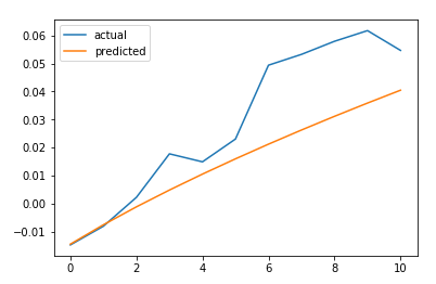
结论
LSTM不能解决时间序列预测问题。对一个时间步长的预测并不比滞后模型好多少。如果我们增加预测的时间步长,性能下降的速度就不会像其他更传统的方法那么快。然而,在这种情况下,我们的误差增加了大约4.5倍。它随着我们试图预测的时间步长呈超线性增长。
