Python_ML_斯坦福机器学习笔记

 

 

斯坦福机器学习笔记

1. Introduction
2. 线性回归
   1. 回归问题
   2. 线性回归与梯度下降
   3. 程序示例--梯度下降
   4. 正规方程
   5. 特征缩放
   6. 多项式回归
   7. 程序示例--多项式回归
   8. 欠拟合与过拟合
   9. 程序示例--局部加权线性回归
3. 逻辑回归
   1. 0/1 分类问题
   2. 逻辑回归
   3. 利用正规化解决过拟合问题
   4. 程序示例--线性决策边界
   5. 程序示例--非线性决策边界
   6. 多分类问题
   7. 程序示例--多分类问题
4. 神经网络
   1. 再论 0/1 分类问题
   2. 神经网络概述
   3. 前向传播与反向传播
   4. 参数展开
   5. 梯度校验
   6. 权值初始化
   7. 感知器
   8. 神经网络解决逻辑运算问题
   9. 神经网络解决多分类问题
   10. 程序示例--神经网络设计
   11. 程序示例--逻辑运算
   12. 程序示例--多分类问题
5. 算法分析与优化
   1. 陷入不归路的调试
   2. 数据集划分
   3. 偏差与方差
   4. 机器学习系统设计--垃圾邮件分类
   5. 偏斜类
   6. 大数据集
   7. 程序示例--算法诊断
6. SVM（支持向量机）
   1. 代价函数
   2. 大间距分类器
   3. 核函数
   4. SVM 的使用建议
   5. SVM 补充
   6. SMO
   7. 程序示例--基于 SMO 的 SVM 模型
   8. 程序示例--线性分类
   9. 程序示例--非线性分类
   10. 程序示例--模型选择
   11. 程序示例--垃圾邮件检测
7. K-Means
   1. 无监督学习
   2. K-Means 算法步骤
   3. 优化
   4. 如何初始化聚类中心
   5. 如何确定聚类数
   6. 二分 K-Means 算法
   7. 程序示例--K-Means
   8. 程序示例--二分 K-Means
8. 特征降维
   1. 概述
   2. PCA
   3. 程序示例--PCA 模型
   4. 程序示例--PCA for 加速学习
   5. 程序示例--PCA for 数据可视化
9. 异常检测
   1. 概述
   2. 高斯分布模型
   3. 算法流程与评估
   4. 有监督学习与异常检测
   5. 特征选择
   6. 多元高斯分布模型
   7. 程序示例--异常检测
10. 推荐系统
    1. 基于内容的推荐系统
    2. 协同过滤
    3. 低秩矩阵分解
    4. 均值标准化
    5. 程序示例--推荐系统
11. 大规模机器学习
    1. 掌握大数据
    2. 梯度下降
    3. 在线学习与MapReduce
12. 案例--光学字符识别
    1. 问题描述及算法流程
    2. 滑动窗口
    3. 人工合成数据
    4. 上限分析
13. 本書使用 GitBook 釋出

 

1. Introduction 

斯坦福机器学习笔记

本书为斯坦福吴恩达教授的在 coursera 上的机器学习公开课的知识笔记，涵盖了大部分课上涉及到的知识点和内容，因为篇幅有限，部分公式的推导没有记录在案，但推荐大家还是在草稿本上演算一遍，加深印象，知其然还要知其所以然。

本书涉及到的程序代码均放在了我个人的 github 上，采用了 python 实现，大部分代码都是相关学习算法的完整实现和测试。我没有放这门课程的 homework 代码，原因是 homework 布置的编程作业是填空式的作业，而完整实现一个算法虽然历经更多坎坷，但更有助于检验自己对算法理解和掌握程度。

本书的章节安排与课程对应关系为：

 

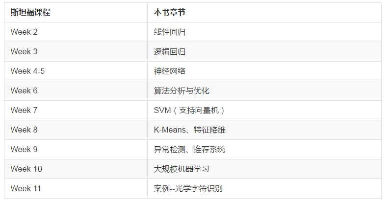
2. 线性回归

2.1 回归问题

假定我们现有一大批数据，包含房屋的面积和对应面积的房价信息，如果我们能得到房屋面积与房屋价格间的关系，那么，给定一个房屋时，我们只要知道其面积，就能大致推测出其价格了。

上面的问题还可以被描述为：

“OK，我具备了很多关于房屋面积及其对应售价的知识（数据），再通过一定的学习，当面对新的房屋面积时，我不再对其定价感到束手无策”。

通常，这类预测问题可以用回归模型（regression）进行解决，回归模型定义了输入与输出的关系，输入即现有知识，而输出则为预测。

一个预测问题在回归模型下的解决步骤为：

1. 积累知识： 我们将储备的知识称之为训练集 Training Set，很好理解，知识能够训练人进步
2. 学习：学习如何预测，得到输入与输出的关系。在学习阶段，应当有合适的指导方针，江山不能仅凭热血就攻下。在这里，合适的指导方针我们称之为学习算法 Learning Algorithm
3. 预测：学习完成后，当接受了新的数据（输入）后，我们就能通过学习阶段获得的对应关系来预测输出。

学习过程往往是艰苦的，“人谁无过，过而能改，善莫大焉”，因此对我们有这两点要求：

• 有手段能评估我们的学习正确性。
• 当学习效果不佳时，有手段能纠正我们的学习策略。

 

2.2 线性回归与梯度下降

线性回归

预测

首先，我们明确几个常用的数学符号：

• 特征（feature）：x_i， 比如，房屋的面积，卧室数量都算房屋的特征
• 特征向量（输入）：x，一套房屋的信息就算一个特征向量，特征向量由特征组成，x_j⁽ⁱ⁾ 表示第 i 个特征向量的第 j 个特征。
• 输出向量：y，y⁽ⁱ⁾ 表示了第 i 个输入所对应的输出
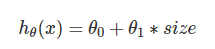
• 假设（hypothesis）：也称为预测函数，比如一个线性预测函数是： 

　　　　h_θ(x)=θ₀+θ₁x₁+θ₂x₂+⋯+θ_nx_n=θ^Tx

上面的表达式也称之为回归方程（regression equation），θ 为回归系数，它是我们预测准度的基石。

 

误差评估

之前我们说到，需要某个手段来评估我们的学习效果，即评估各个真实值 y⁽ⁱ⁾ 与预测值 h_θ(x⁽ⁱ⁾) 之间的差异。最常见的，我们通过最小均方（Least Mean Square）来描述误差：

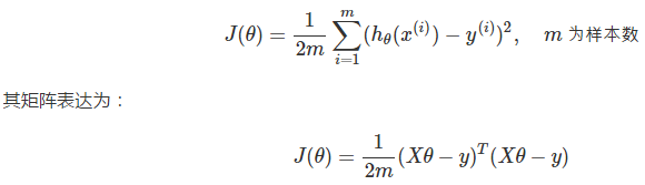
误差评估的函数在机器学习中也称为代价函数（cost function）。

 

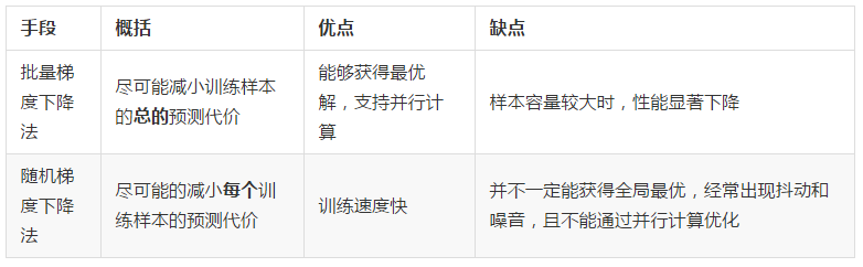
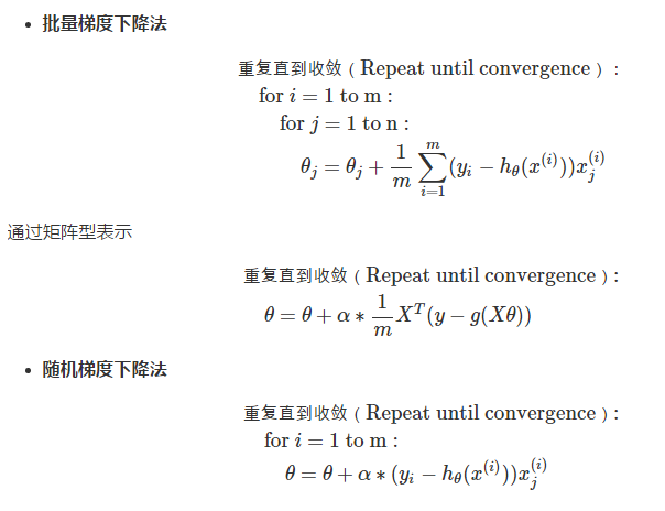
批量梯度下降

在引入了代价函数后，解决了“有手段评估学习的正确性”的问题，下面我们开始解决“当学习效果不佳时，有手段能纠正我们的学习策略”的问题。

首先可以明确的是，该手段就是要反复调节 θ 是的预测 J(θ) 足够小，以及使得预测精度足够高，在线性回归中，通常使用梯度下降（Gradient Descent）来调节 θ：

 　　　　　　　　　　

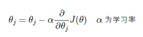
数学上，梯度方向是函数值下降最为剧烈的方向。那么，沿着 J(θ) 的梯度方向走，我们就能接近其最小值，或者极小值，从而接近更高的预测精度。学习率 α 是个相当玄乎的参数，其标识了沿梯度方向行进的速率，步子大了容易扯着蛋，很可能这一步就迈过了最小值。而步子小了，又会减缓我们找到最小值的速率。在实际编程中，学习率可以以 3 倍，10 倍这样进行取值尝试，如：

　　　　　　　　　　 α=0.001,0.003,0.01…0.3,1

对于一个样本容量为 mm 的训练集，我们定义 θ 的调优过程为： 

　　　重复直到收敛（Repeat until convergence）：

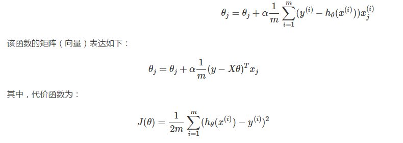
我们称该过程为基于最小均方（LMS）的批量梯度下降法（Batch Gradient Descent），一方面，该方法虽然可以收敛到最小值，但是每调节一个 θj，都不得不遍历一遍样本集，如果样本的体积 m 很大，这样做无疑开销巨大。但另一方面，因为其可化解为向量型表示，所以就能利用到并行计算优化性能。

 

随机梯度下降

鉴于批量梯度下降的性能问题，又引入了随机梯度下降（Stochastic Gradient Descent）：

  

 可以看到，在随机梯度下降法中，每次更新 θj 只需要一个样本：(x(i),y(i))(x(i),y(i))。即便在样本集容量巨大时，我们也很可能迅速获得最优解，此时 SGD 能带来明显的性能提升。

  

2.3 程序示例--梯度下降

回归模块

回归模块中提供了批量梯度下降和随机梯度下降两种学习策略来训练模型：

# coding: utf-8
# linear_regression/regression.py
import numpy as np
import matplotlib as plt
import time

def exeTime(func):
    """ 耗时计算装饰器
    """
    def newFunc(*args, **args2):
        t0 = time.time()
        back = func(*args, **args2)
        return back, time.time() - t0
    return newFunc

def loadDataSet(filename):
    """ 读取数据

    从文件中获取数据，在《机器学习实战中》，数据格式如下
    "feature1 TAB feature2 TAB feature3 TAB label"

    Args:
        filename: 文件名

    Returns:
        X: 训练样本集矩阵
        y: 标签集矩阵
    """
    numFeat = len(open(filename).readline().split('\t')) - 1
    X = []
    y = []
    file = open(filename)
    for line in file.readlines():
        lineArr = []
        curLine = line.strip().split('\t')
        for i in range(numFeat):
            lineArr.append(float(curLine[i]))
        X.append(lineArr)
        y.append(float(curLine[-1]))
    return np.mat(X), np.mat(y).T

def h(theta, x):
    """预测函数

    Args:
        theta: 相关系数矩阵
        x: 特征向量

    Returns:
        预测结果
    """
    return (theta.T*x)[0,0]

def J(theta, X, y):
    """代价函数

    Args:
        theta: 相关系数矩阵
        X: 样本集矩阵
        y: 标签集矩阵

    Returns:
        预测误差（代价）
    """
    m = len(X)
    return (X*theta-y).T*(X*theta-y)/(2*m)

@exeTime
def bgd(rate, maxLoop, epsilon, X, y):
    """批量梯度下降法

    Args:
        rate: 学习率
        maxLoop: 最大迭代次数
        epsilon: 收敛精度
        X: 样本矩阵
        y: 标签矩阵

    Returns:
        (theta, errors, thetas), timeConsumed
    """
    m,n = X.shape
    # 初始化theta
    theta = np.zeros((n,1))
    count = 0
    converged = False
    error = float('inf')
    errors = []
    thetas = {}
    for j in range(n):
        thetas[j] = [theta[j,0]]
    while count<=maxLoop:
        if(converged):
            break
        count = count + 1
        for j in range(n):
            deriv = (y-X*theta).T*X[:, j]/m
            theta[j,0] = theta[j,0]+rate*deriv
            thetas[j].append(theta[j,0])
        error = J(theta, X, y)
        errors.append(error[0,0])
        # 如果已经收敛
        if(error < epsilon):
            converged = True
    return theta,errors,thetas

@exeTime
def sgd(rate, maxLoop, epsilon, X, y):
    """随机梯度下降法
    Args:
        rate: 学习率
        maxLoop: 最大迭代次数
        epsilon: 收敛精度
        X: 样本矩阵
        y: 标签矩阵
    Returns:
        (theta, error, thetas), timeConsumed
    """
    m,n = X.shape
    # 初始化theta
    theta = np.zeros((n,1))
    count = 0
    converged = False
    error = float('inf')
    errors = []
    thetas = {}
    for j in range(n):
        thetas[j] = [theta[j,0]]
    while count <= maxLoop:
        if(converged):
            break
        count = count + 1
        errors.append(float('inf'))
        for i in range(m):
            if(converged):
                break
            diff = y[i,0]-h(theta, X[i].T)
            for j in range(n):
                theta[j,0] = theta[j,0] + rate*diff*X[i, j]
                thetas[j].append(theta[j,0])
            error = J(theta, X, y)
            errors[-1] = error[0,0]
            # 如果已经收敛
            if(error < epsilon):
                converged = True
    return theta, errors, thetas

 

测试程序

bgd测试程序

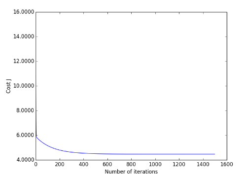
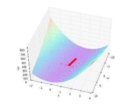
# coding: utf-8
# linear_regression/test_bgd.py
import regression
from matplotlib import cm
from mpl_toolkits.mplot3d import axes3d
import matplotlib.pyplot as plt
import matplotlib.ticker as mtick
import numpy as np

if **name** == "**main**":
    X, y = regression.loadDataSet('data/ex1.txt');

    m,n = X.shape
    X = np.concatenate((np.ones((m,1)), X), axis=1)

    rate = 0.01
    maxLoop = 1500
    epsilon =0.01

    result, timeConsumed = regression.bgd(rate, maxLoop, epsilon, X, y)

    theta, errors, thetas = result

    # 绘制拟合曲线
    fittingFig = plt.figure()
    title = 'bgd: rate=%.2f, maxLoop=%d, epsilon=%.3f \n time: %ds'%(rate,maxLoop,epsilon,timeConsumed)
    ax = fittingFig.add_subplot(111, title=title)
    trainingSet = ax.scatter(X[:, 1].flatten().A[0], y[:,0].flatten().A[0])

    xCopy = X.copy()
    xCopy.sort(0)
    yHat = xCopy*theta
    fittingLine, = ax.plot(xCopy[:,1], yHat, color='g')

    ax.set_xlabel('Population of City in 10,000s')
    ax.set_ylabel('Profit in $10,000s')

    plt.legend([trainingSet, fittingLine], ['Training Set', 'Linear Regression'])
    plt.show()

    # 绘制误差曲线
    errorsFig = plt.figure()
    ax = errorsFig.add_subplot(111)
    ax.yaxis.set_major_formatter(mtick.FormatStrFormatter('%.4f'))

    ax.plot(range(len(errors)), errors)
    ax.set_xlabel('Number of iterations')
    ax.set_ylabel('Cost J')

    plt.show()

    # 绘制能量下降曲面
    size = 100
    theta0Vals = np.linspace(-10,10, size)
    theta1Vals = np.linspace(-2, 4, size)
    JVals = np.zeros((size, size))
    for i in range(size):
        for j in range(size):
            col = np.matrix([[theta0Vals[i]], [theta1Vals[j]]])
            JVals[i,j] = regression.J(col, X, y)

    theta0Vals, theta1Vals = np.meshgrid(theta0Vals, theta1Vals)
    JVals = JVals.T
    contourSurf = plt.figure()
    ax = contourSurf.gca(projection='3d')

    ax.plot_surface(theta0Vals, theta1Vals, JVals,  rstride=2, cstride=2, alpha=0.3,
                cmap=cm.rainbow, linewidth=0, antialiased=False)
    ax.plot(thetas[0], thetas[1], 'rx')
    ax.set_xlabel(r'$\theta_0$')
    ax.set_ylabel(r'$\theta_1$')
    ax.set_zlabel(r'$J(\theta)$')

    plt.show()

    # 绘制能量轮廓
    contourFig = plt.figure()
    ax = contourFig.add_subplot(111)
    ax.set_xlabel(r'$\theta_0$')
    ax.set_ylabel(r'$\theta_1$')

    CS = ax.contour(theta0Vals, theta1Vals, JVals, np.logspace(-2,3,20))
    plt.clabel(CS, inline=1, fontsize=10)

    # 绘制最优解
    ax.plot(theta[0,0], theta[1,0], 'rx', markersize=10, linewidth=2)

    # 绘制梯度下降过程
    ax.plot(thetas[0], thetas[1], 'rx', markersize=3, linewidth=1)
    ax.plot(thetas[0], thetas[1], 'r-')

    plt.show()

 

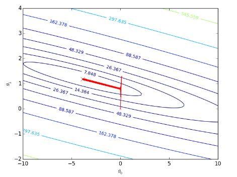
拟合状况：

 

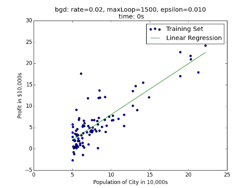
可以看到，bgd 运行的并不慢，这是因为在 regression 程序中，我们采用了向量形式计算 θ，计算机会通过并行计算的手段来优化速度。

误差随迭代次数的关系：

 

误差函数的下降曲面：

 

梯度下架过程：

 

sgd测试：

# coding: utf-8
# linear_regression/test_sgd.py
import regression
from matplotlib import cm
from mpl_toolkits.mplot3d import axes3d
import matplotlib.pyplot as plt
import matplotlib.ticker as mtick
import numpy as np

if **name** == "**main**":
    X, y = regression.loadDataSet('data/ex1.txt');

    m,n = X.shape
    X = np.concatenate((np.ones((m,1)), X), axis=1)

    rate = 0.01
    maxLoop = 100
    epsilon =0.01

    result, timeConsumed = regression.sgd(rate, maxLoop, epsilon, X, y)

    theta, errors, thetas = result

    # 绘制拟合曲线
    fittingFig = plt.figure()
    title = 'sgd: rate=%.2f, maxLoop=%d, epsilon=%.3f \n time: %ds'%(rate,maxLoop,epsilon,timeConsumed)
    ax = fittingFig.add_subplot(111, title=title)
    trainingSet = ax.scatter(X[:, 1].flatten().A[0], y[:,0].flatten().A[0])

    xCopy = X.copy()
    xCopy.sort(0)
    yHat = xCopy*theta
    fittingLine, = ax.plot(xCopy[:,1], yHat, color='g')

    ax.set_xlabel('Population of City in 10,000s')
    ax.set_ylabel('Profit in $10,000s')

    plt.legend([trainingSet, fittingLine], ['Training Set', 'Linear Regression'])
    plt.show()

    # 绘制误差曲线
    errorsFig = plt.figure()
    ax = errorsFig.add_subplot(111)
    ax.yaxis.set_major_formatter(mtick.FormatStrFormatter('%.4f'))

    ax.plot(range(len(errors)), errors)
    ax.set_xlabel('Number of iterations')
    ax.set_ylabel('Cost J')

    plt.show()

    # 绘制能量下降曲面
    size = 100
    theta0Vals = np.linspace(-10,10, size)
    theta1Vals = np.linspace(-2, 4, size)
    JVals = np.zeros((size, size))
    for i in range(size):
        for j in range(size):
            col = np.matrix([[theta0Vals[i]], [theta1Vals[j]]])
            JVals[i,j] = regression.J(col, X, y)

    theta0Vals, theta1Vals = np.meshgrid(theta0Vals, theta1Vals)
    JVals = JVals.T
    contourSurf = plt.figure()
    ax = contourSurf.gca(projection='3d')

    ax.plot_surface(theta0Vals, theta1Vals, JVals,  rstride=8, cstride=8, alpha=0.3,
                cmap=cm.rainbow, linewidth=0, antialiased=False)
    ax.plot(thetas[0], thetas[1], 'rx')
    ax.set_xlabel(r'$\theta_0$')
    ax.set_ylabel(r'$\theta_1$')
    ax.set_zlabel(r'$J(\theta)$')

    plt.show()

    # 绘制能量轮廓
    contourFig = plt.figure()
    ax = contourFig.add_subplot(111)
    ax.set_xlabel(r'$\theta_0$')
    ax.set_ylabel(r'$\theta_1$')

    CS = ax.contour(theta0Vals, theta1Vals, JVals, np.logspace(-2,3,20))
    plt.clabel(CS, inline=1, fontsize=10)

    # 绘制最优解
    ax.plot(theta[0,0], theta[1,0], 'rx', markersize=10, linewidth=2)

    # 绘制梯度下降过程
    ax.plot(thetas[0], thetas[1], 'r', linewidth=1)

    plt.show()

 

 拟合状况：

误差随迭代次数的关系：

梯度下降过程：

在学习率为 0.010.01 时，随机梯度下降法出现了非常明显的抖动，同时，随机梯度下降法的速度优势也并未在此得到体现，一是样本容量不大，二是其自身很难通过并行计算去优化速度。 

 

2.4 正规方程（Normal Equation）

定义

前面论述的线性回归问题中，我们通过梯度下降法来求得 J(θ) 的最小值，但是对于学习率 α 的调节有时候使得我们非常恼火。为此，我们可通过正规方程来最小化 J(θ)：

 　　　　　　　　　　　　

其中，X 为输入向量矩阵，第 0 个特征表示偏置（x₀=1），y 为目标向量，仅从该表达式形式上看，我们也脱离了学习率 α 的束缚。

梯度下降与正规方程的对比

  

2.5 特征缩放

引子

在前一章节中，对房屋售价进行预测时，我们的特征仅有房屋面积一项，但是，在实际生活中，卧室数目也一定程度上影响了房屋售价。下面，我们有这样一组训练样本

 

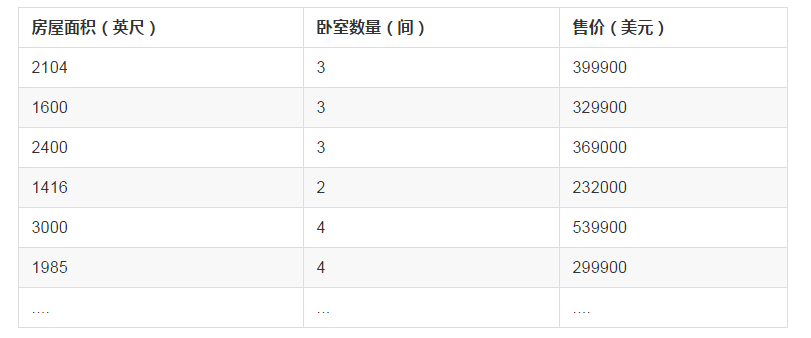
注意到，房屋面积及卧室数量两个特征在数值上差异巨大，如果直接将该样本送入训练，则代价函数的轮廓会是“扁长的”，在找到最优解前，梯度下降的过程不仅是曲折的，也是非常耗时的：

缩放

该问题的出现是因为我们没有同等程度的看待各个特征，即我们没有将各个特征量化到统一的区间。量化的方式有如下两种：

Standardization

Standardization 又称为 Z-score normalization，量化后的特征将服从标准正态分布：

 

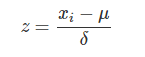
其中，μ，δ 分别为对应特征 xi 的均值和标准差。量化后的特征将分布在 [−1,1] 区间。

Min-Max Scaling

Min-Max Scaling 又称为 normalization，特征量化的公式为：

 

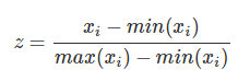
量化后的特征将分布在 [0,1][0,1] 区间。

大多数机器学习算法中，会选择 Standardization 来进行特征缩放，但是，Min-Max Scaling 也并非会被弃置一地。在数字图像处理中，像素强度通常就会被量化到 [0,1][0,1] 区间，在一般的神经网络算法中，也会要求特征被量化到 [0,1][0,1] 区间。

进行了特征缩放以后，代价函数的轮廓会是“偏圆”的，梯度下降过程更加笔直，性能因此也得到提升：

实现

在 regression.py 中，我们添加了 Standardization 和 Normalization 的实现：

# linear_regression/regression.py

# ...
def standardize(X):
    """特征标准化处理

    Args:
        X: 样本集
    Returns:
        标准后的样本集
    """
    m, n = X.shape
    # 归一化每一个特征
    for j in range(n):
        features = X[:,j]
        meanVal = features.mean(axis=0)
        std = features.std(axis=0)
        if std != 0:
            X[:, j] = (features-meanVal)/std
        else
            X[:, j] = 0
    return X

def normalize(X):
    """特征归一化处理

    Args:
        X: 样本集
    Returns:
        归一化后的样本集
    """
    m, n = X.shape
    # 归一化每一个特征
    for j in range(n):
        features = X[:,j]
        minVal = features.min(axis=0)
        maxVal = features.max(axis=0)
        diff = maxVal - minVal
        if diff != 0:
           X[:,j] = (features-minVal)/diff
        else:
           X[:,j] = 0
    return X
# ...

 

参考文献

• About Feature Scaling and Normalization
• Wiki--Feature scaling

 

2.6 多项式回归

在线性回归中，我们通过如下函数来预测对应房屋面积的房价：

　　　　

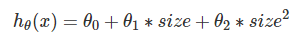
通过程序我们也知道，该函数得到的是直线拟合，精度欠佳。现在，我们可以考虑对房价特征 size 进行平方，以及获得更加精准的 size 变化：

　　　　

这就是多项式回归。

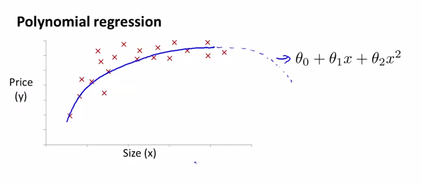
如下图所示，多项式回归得到了更好的拟合曲线。但我们也发现，在房屋面积足够大时，曲线反而出现了下沿，这意味着房价反而随着在房屋面积足够大时，与面积成反比，这明显不符合可观规律（虽然我们很渴望这样的情况出现）：

 

进一步地，我们考虑加上三次方项目或者替换二次方项为开方，得到如下两种预测：

 　　　　

 

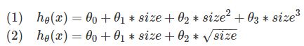
 在该例中，因为三次方项会带来很大的值，所以优先考虑采用了开方的预测函数。

 

2.7 程序示例--多项式回归

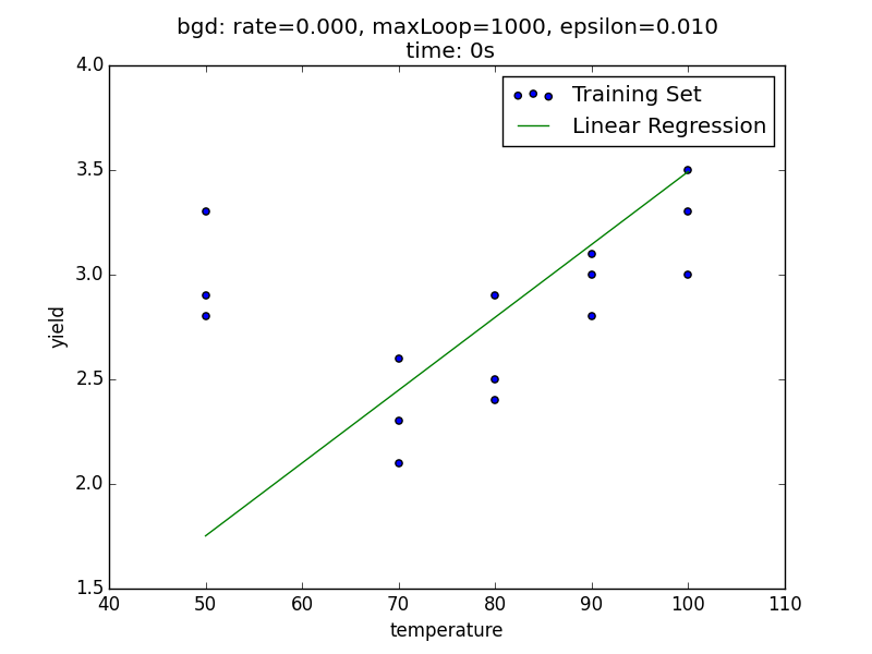
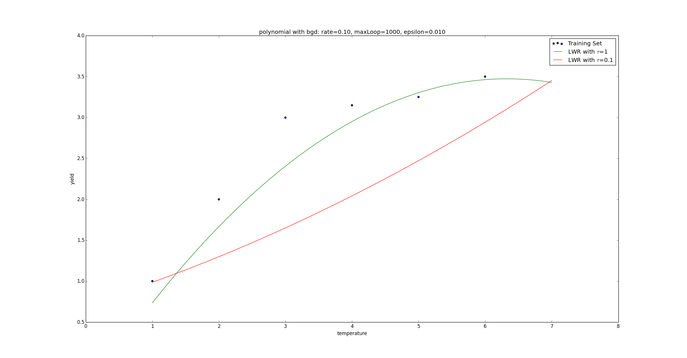
下面，我们有一组温度（temperature）和实验产出量（yield）训练样本，该数据由博客 Polynomial Regression Examples 所提供：

我们先通过如下预测函数进行训练：

　　　　h(θ)=θ₀+θ₁x

# coding: utf-8
# linear_regression/test_temperature_normal.py
import regression
from matplotlib import cm
from mpl_toolkits.mplot3d import axes3d
import matplotlib.pyplot as plt
import matplotlib.ticker as mtick
import numpy as np

if __name__ == "__main__":
    X, y = regression.loadDataSet('data/temperature.txt');

    m,n = X.shape
    X = np.concatenate((np.ones((m,1)), X), axis=1)

    rate = 0.0001
    maxLoop = 1000
    epsilon =0.01

    result, timeConsumed = regression.bgd(rate, maxLoop, epsilon, X, y)

    theta, errors, thetas = result

    # 绘制拟合曲线
    fittingFig = plt.figure()
    title = 'bgd: rate=%.3f, maxLoop=%d, epsilon=%.3f \n time: %ds'%(rate,maxLoop,epsilon,timeConsumed)
    ax = fittingFig.add_subplot(111, title=title)
    trainingSet = ax.scatter(X[:, 1].flatten().A[0], y[:,0].flatten().A[0])

    xCopy = X.copy()
    xCopy.sort(0)
    yHat = xCopy*theta
    fittingLine, = ax.plot(xCopy[:,1], yHat, color='g')

    ax.set_xlabel('temperature')
    ax.set_ylabel('yield')

    plt.legend([trainingSet, fittingLine], ['Training Set', 'Linear Regression'])
    plt.show()

    # 绘制误差曲线
    errorsFig = plt.figure()
    ax = errorsFig.add_subplot(111)
    ax.yaxis.set_major_formatter(mtick.FormatStrFormatter('%.4f'))

    ax.plot(range(len(errors)), errors)
    ax.set_xlabel('Number of iterations')
    ax.set_ylabel('Cost J')

    plt.show()

得到的拟合图像为：

接下来，我们使用了多项式回归，添加了 2 阶项：

　　　　 

 因为 x 与 x² 数值差异较大，所以我们会先做一次特征标准化，将各个特征缩放到 [−1,1] 区间

 　　　　　　

得到的拟合曲线更加准确：

# coding: utf-8
# linear_regression/test_temperature_polynomial.py

import regression
import matplotlib.pyplot as plt
import matplotlib.ticker as mtick
import numpy as np

if __name__ == "__main__":
    srcX, y = regression.loadDataSet('data/temperature.txt');

    m,n = srcX.shape
    srcX = np.concatenate((srcX[:, 0], np.power(srcX[:, 0],2)), axis=1)
    # 特征缩放
    X = regression.standardize(srcX.copy())
    X = np.concatenate((np.ones((m,1)), X), axis=1)

    rate = 0.1
    maxLoop = 1000
    epsilon = 0.01

    result, timeConsumed = regression.bgd(rate, maxLoop, epsilon, X, y)
    theta, errors, thetas = result

    # 打印特征点
    fittingFig = plt.figure()
    title = 'polynomial with bgd: rate=%.2f, maxLoop=%d, epsilon=%.3f \n time: %ds'%(rate,maxLoop,epsilon,timeConsumed)
    ax = fittingFig.add_subplot(111, title=title)
    trainingSet = ax.scatter(srcX[:, 1].flatten().A[0], y[:,0].flatten().A[0])

    print theta

    # 打印拟合曲线
    xx = np.linspace(50,100,50)
    xx2 = np.power(xx,2)
    yHat = []
    for i in range(50):
        normalizedSize = (xx[i]-xx.mean())/xx.std(0)
        normalizedSize2 = (xx2[i]-xx2.mean())/xx2.std(0)
        x = np.matrix([[1,normalizedSize, normalizedSize2]])
        yHat.append(regression.h(theta, x.T))
    fittingLine, = ax.plot(xx, yHat, color='g')

    ax.set_xlabel('Yield')
    ax.set_ylabel('temperature')

    plt.legend([trainingSet, fittingLine], ['Training Set', 'Polynomial Regression'])
    plt.show()

    # 打印误差曲线
    errorsFig = plt.figure()
    ax = errorsFig.add_subplot(111)
    ax.yaxis.set_major_formatter(mtick.FormatStrFormatter('%.2e'))

    ax.plot(range(len(errors)), errors)
    ax.set_xlabel('Number of iterations')
    ax.set_ylabel('Cost J')

    plt.show()

 

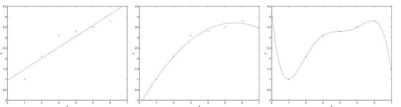
2.8 欠拟合与过拟合

问题

在上一节中，我们利用多项式回归获得更加准确的拟合曲线，实现了对训练数据更好的拟合。然而，我们也发现，过渡地对训练数据拟合也会丢失信息规律。首先，引出两个概念：

• 欠拟合（underfitting）：拟合程度不高，数据距离拟合曲线较远，如下左图所示。

• 过拟合（overfitting）：过度拟合，貌似拟合几乎每一个数据，但是丢失了信息规律，如下右图所示，房价随着房屋面积的增加反而降低了。

　　　　　　 

局部加权线性回归（LWR）

为了解决欠拟合和过拟合问题，引入了局部加权线性回归（Locally Weight Regression）。在一般的线性回归算法中，对于某个输入向量 x，我们这样预测输出 y： 

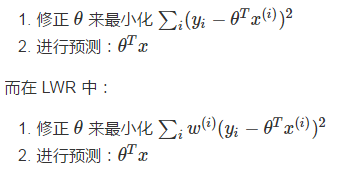
在 LWR 中，我们对一个输入 x 进行预测时，赋予了 x 周围点不同的权值，距离 x 越近，权重越高。整个学习过程中误差将会取决于 x 周围的误差，而不是整体的误差，这也就是局部一词的由来。

通常，w⁽ⁱ⁾ 服从高斯分布，在 x 周围呈指数型衰减：

　　　　　　　　 

其中，τ 值越小，则靠近预测点的权重越大，而远离预测点的权重越小。

另外，LWR 属于非参数（non-parametric）学习算法，所谓的非参数学习算法指的是没有明确的参数（比如上述的 θ 取决于当前要预测的 x），每进行一次预测，就需要重新进行训练。而一般的线性回归属于参数（parametric）学习算法，参数在训练后将不再改变。 

LWR 补充自机器学习实战一书，后续章节中我们知道，更一般地，我们使用正规化来解决过拟合问题。

 

2.9 程序示例--局部加权线性回归

现在，我们在回归中又添加了 JLwr() 方法用于计算预测代价，以及 lwr() 方法用于完成局部加权线性回归：

# coding: utf-8
# linear_regression/regression.py

# ...

def JLwr(theta, X, y, x, c):
    """局部加权线性回归的代价函数计算式

    Args:
        theta: 相关系数矩阵
        X: 样本集矩阵
        y: 标签集矩阵
        x: 待预测输入
        c: tau
    Returns:
        预测代价
    """
    m,n = X.shape
    summerize = 0
    for i in range(m):
        diff = (X[i]-x)*(X[i]-x).T
        w = np.exp(-diff/(2*c*c))
        predictDiff = np.power(y[i] - X[i]*theta,2)
        summerize = summerize + w*predictDiff
    return summerize

@exeTime
def lwr(rate, maxLoop, epsilon, X, y, x, c=1):
    """局部加权线性回归

    Args:
        rate: 学习率
        maxLoop: 最大迭代次数
        epsilon: 预测精度
        X: 输入样本
        y: 标签向量
        x: 待预测向量
        c: tau
    """
    m,n = X.shape
    # 初始化theta
    theta = np.zeros((n,1))
    count = 0
    converged = False
    error = float('inf')
    errors = []
    thetas = {}
    for j in range(n):
        thetas[j] = [theta[j,0]]
    # 执行批量梯度下降
    while count<=maxLoop:
        if(converged):
            break
        count = count + 1
        for j in range(n):
            deriv = (y-X*theta).T*X[:, j]/m
            theta[j,0] = theta[j,0]+rate*deriv
            thetas[j].append(theta[j,0])
        error = JLwr(theta, X, y, x, c)
        errors.append(error[0,0])
        # 如果已经收敛
        if(error < epsilon):
            converged = True
    return theta,errors,thetas

# ...

 

测试：

# coding: utf-8
# linear_regression/test_lwr.py
import regression
import matplotlib.pyplot as plt
import matplotlib.ticker as mtick
import numpy as np

if __name__ == "__main__":
    srcX, y = regression.loadDataSet('data/lwr.txt');

    m,n = srcX.shape
    srcX = np.concatenate((srcX[:, 0], np.power(srcX[:, 0],2)), axis=1)
    # 特征缩放
    X = regression.standardize(srcX.copy())
    X = np.concatenate((np.ones((m,1)), X), axis=1)

    rate = 0.1
    maxLoop = 1000
    epsilon = 0.01

    predicateX = regression.standardize(np.matrix([[8, 64]]))

    predicateX = np.concatenate((np.ones((1,1)), predicateX), axis=1)

    result, t = regression.lwr(rate, maxLoop, epsilon, X, y, predicateX, 1)
    theta, errors, thetas = result

    result2, t = regression.lwr(rate, maxLoop, epsilon, X, y, predicateX, 0.1)
    theta2, errors2, thetas2 = result2


    # 打印特征点
    fittingFig = plt.figure()
    title = 'polynomial with bgd: rate=%.2f, maxLoop=%d, epsilon=%.3f'%(rate,maxLoop,epsilon)
    ax = fittingFig.add_subplot(111, title=title)
    trainingSet = ax.scatter(srcX[:, 0].flatten().A[0], y[:,0].flatten().A[0])

    print theta
    print theta2

    # 打印拟合曲线
    xx = np.linspace(1, 7, 50)
    xx2 = np.power(xx,2)
    yHat1 = []
    yHat2 = []
    for i in range(50):
        normalizedSize = (xx[i]-xx.mean())/xx.std(0)
        normalizedSize2 = (xx2[i]-xx2.mean())/xx2.std(0)
        x = np.matrix([[1,normalizedSize, normalizedSize2]])
        yHat1.append(regression.h(theta, x.T))
        yHat2.append(regression.h(theta2, x.T))
    fittingLine1, = ax.plot(xx, yHat1, color='g')
    fittingLine2, = ax.plot(xx, yHat2, color='r')

    ax.set_xlabel('temperature')
    ax.set_ylabel('yield')

    plt.legend([trainingSet, fittingLine1, fittingLine2], ['Training Set', r'LWR with $\tau$=1', r'LWR with $\tau$=0.1'])
    plt.show()

    # 打印误差曲线
    errorsFig = plt.figure()
    ax = errorsFig.add_subplot(111)
    ax.yaxis.set_major_formatter(mtick.FormatStrFormatter('%.2e'))

    ax.plot(range(len(errors)), errors)
    ax.set_xlabel('Number of iterations')
    ax.set_ylabel('Cost J')

    plt.show()

在测试程序中，我们分别对 ττ 取值 0.10.1 和 11，得到了不同的拟合曲线：

 

 

3. 逻辑回归

3.1 0/1 分类问题

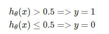
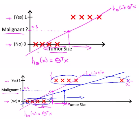
利用线性回归中的预测函数 hθ(x)，我们定义阈值函数来完成 0/1 分类：

　　 

下面两幅图展示了线性预测。在第一幅图中，拟合曲线成功的区分了 0、1 两类，在第二幅图中，如果我们新增了一个输入（右上的 X 所示），此时拟合曲线发生变化，由第一幅图中的紫色线旋转到第二幅图的蓝色线，导致本应被视作 1 类的 X 被误分为了 0 类：

 

3.2 逻辑回归

逻辑回归

上一节我们知道，使用线性回归来处理 0/1 分类问题总是困难重重的，因此，人们定义了逻辑回归来完成 0/1 分类问题，逻辑一词也代表了是（1）和非（0）。

Sigmoid预测函数

在逻辑回归中，定义预测函数为：

 　　　　　　hθ(x)=g(z)

其中，z=θ^Tx 是分类边界，且 g(z)=1/（1+e^−z）。

g(z) 称之为 Sigmoid Function，亦称 Logic Function，其函数图像如下：

 

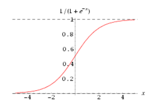
可以看到，预测函数 hθ(x) 被很好地限制在了 0、1 之间，并且，sigmoid 是一个非常好的阈值函数：阈值为 0.5，大于 0.5 为 1 类，反之为 0 类。函数曲线过渡光滑自然，关于 0.5 中心对称也极具美感。

决策边界

决策边界，顾名思义，就是用来划清界限的边界，边界的形态可以不定，可以是点，可以是线，也可以是平面。Andrew Ng 在公开课中强调：“决策边界是预测函数 hθ(x) 的属性，而不是训练集属性”，这是因为能作出“划清”类间界限的只有 hθ(x)，而训练集只是用来训练和调节参数的。

 

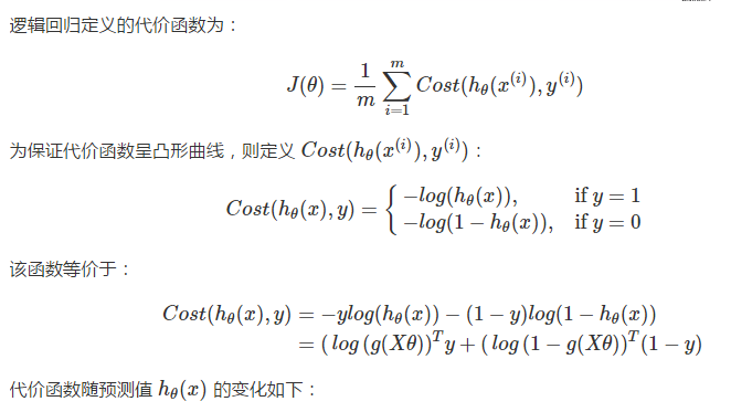
预测代价函数

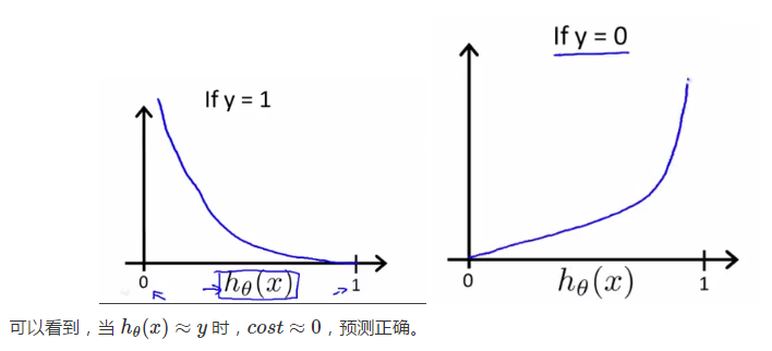
对于分类任务来说，我们就是要反复调节参数 θ，亦即反复转动决策边界来作出更精确的预测。假定我们有代价函数 J(θ)，其用来评估某个 θθ 值时的预测精度，当找到代价函数的最小值时，就能作出最准确的预测。通常，代价函数具备越少的极小值，就越容易找到其最小值，也就越容易达到最准确的预测。

下面两幅图中，左图这样犬牙差互的代价曲线（非凸函数）显然会使我们在做梯度下降的时候陷入迷茫，任何一个极小值都有可能被错认为最小值，但无法获得最优预测精度。但在右图的代价曲线中，就像滑梯一样，我们就很容易达到最小值：

 

 

最小化代价函数

与线性回归一样，也使用梯度下降法来最小化代价函数：

 

3.3 利用正规化解决过拟合问题

在之前的文章中，我们认识了过拟合问题,通常，我们有如下策略来解决过拟合问题：

1. 减少特征数，显然这只是权宜之计，因为特征意味着信息，放弃特征也就等同于丢弃信息，要知道，特征的获取往往也是艰苦卓绝的。

2. 不放弃特征，而是拉伸曲线使之更加平滑以解决过拟合问题，为了拉伸曲线，也就要弱化一些高阶项（曲线曲折的罪魁祸首）。由于高阶项中的特征 x 无法更改，因此特征是无法弱化的，我们能弱化的只有高阶项中的系数 θi。我们把这种弱化称之为是对参数 θ 的惩罚（penalize）。Regularization（正规化）正是完成这样一种惩罚的“侩子手”。

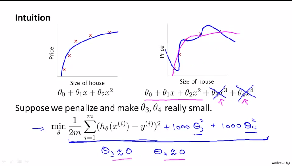
如下例所示，我们将 θ3 及 θ4 减小（惩罚）到趋近于 0，原本过拟合的曲线就变得更加平滑，趋近于一条二次曲线（在本例中，二次曲线显然更能反映住房面积和房价的关系），也就能够更好的根据住房面积来预测房价。要知道，预测才是我们的最终目的，而非拟合。

 

 

线性回归中的正规化

在线性回归中，我们的预测代价如下评估：

 　　

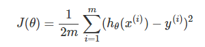
为了在最小化 J(θ) 的过程中，也能尽可能使 θ 变小，我们将上式更改为:

 　　

其中，参数 λλ 主要是完成以下两个任务:

1. 保证对数据的拟合良好
2. 保证 θθ 足够小，避免过拟合问题。

λλ 越大，要使 J(θ)J(θ) 变小，惩罚力度就要变大，这样 θθ 会被惩罚得越惨（越小），即要避免过拟合，我们显然应当增大 λλ 的值。

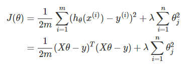
那么，梯度下降也发生相应变化：

其中，（1）式等价于：

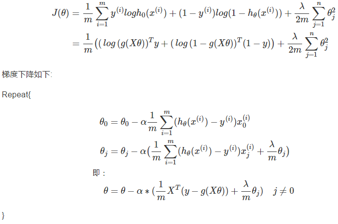
逻辑回归中的正规化

代价评估如下：