
大作业一
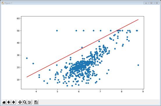
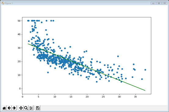
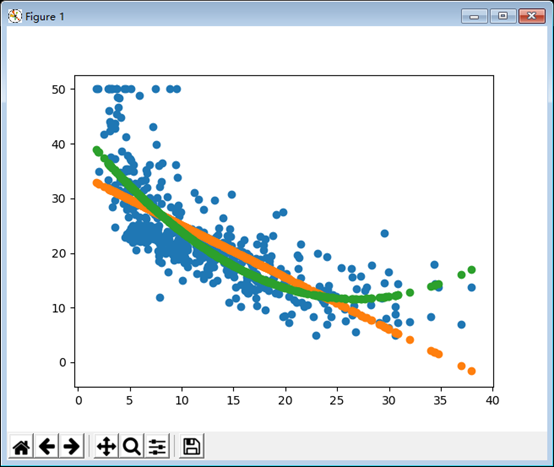
大作业一 boston房价预测
1. 读取数据集
2. 训练集与测试集划分
3. 线性回归模型:建立13个变量与房价之间的预测模型,并检测模型好坏。
4. 多项式回归模型:建立13个变量与房价之间的预测模型,并检测模型好坏。
5. 比较线性模型与非线性模型的性能,并说明原因。


#1.导入boston房价数据集
from sklearn.datasets import load_boston
boston = load_boston()
boston.keys()

print(boston.DESCR)
boston.data.shape
boston.feature_names

import pandas as pd
pd.DataFrame(boston.data)
#2. 一元线性回归模型,建立一个变量与房价之间的预测模型,并图形化显示。
import matplotlib.pyplot as plt
x = boston.data[:,5]
y = boston.target
plt.figure(figsize=(10,6))
plt.scatter(x,y)
plt.plot(x,9*x-20,'r')
plt.show()

from sklearn.linear_model import LinearRegression
lineR=LinearRegression()
lineR.fit(x.reshape(-1,1),y)
w=lineR.coef_
b = lineR.intercept_

#3、多元线性回归模型,建立13个变量与房价之间的预测模型,并检测模型好坏,并图形化显示检查结果
from sklearn.linear_model import LinearRegression
lineR = LinearRegression()
lineR.fit(boston.data,y)
w = lineR.coef_
b = lineR.intercept_

import matplotlib.pyplot as plt
x=boston.data[:,12].reshape(-1,1)
y=boston.target
plt.figure(figsize=(10,6)) #指定显示图大小
plt.scatter(x,y)

from sklearn.linear_model import LinearRegression
lineR=LinearRegression()
lineR.fit(x,y)
y_pred=lineR.predict(x)
plt.plot(x,y_pred,'green')
print(lineR.coef_,lineR.intercept_)
plt.show()

#4.  一元多项式回归模型,建立一个变量与房价之间的预测模型,并图形化显示。
from sklearn.preprocessing import PolynomialFeatures
poly = PolynomialFeatures(degree=2)
x_poly = poly.fit_transform(x)

lrp = LinearRegression()
lrp.fit(x_poly,y)
y_poly_pred = lrp.predict(x_poly)

plt.scatter(x,y)
plt.plot(x,y_poly_pred,'r')
plt.show()

from sklearn.preprocessing import PolynomialFeatures
poly = PolynomialFeatures(degree=2)
x_poly = poly.fit_transform(x)

lrp = LinearRegression()
lrp.fit(x_poly,y)
plt.scatter(x,y)
plt.scatter(x,y_pred)
plt.scatter(x,y_poly_pred)   #多项回归
plt.show()

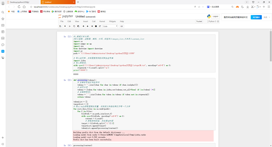
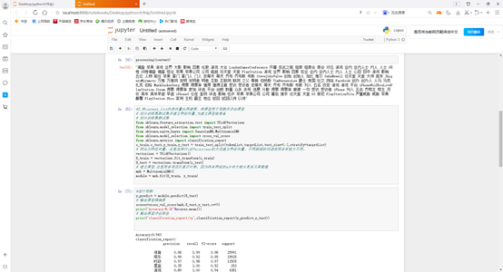
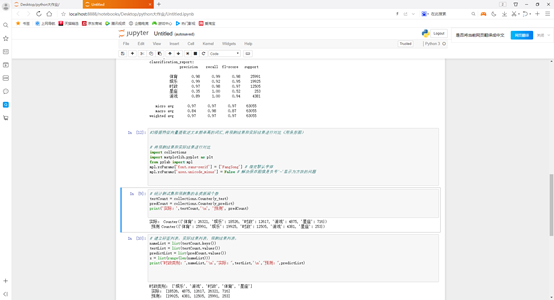
#1.新闻文本分类:
#定义函数:读数据,清洗,分词。标签存入target_list,文本存入content_list
import os
import numpy as np
import sys
from datetime import datetime
import gc
path = 'F:\\计算机\\python\\挖掘\\data'

# 导入结巴库,并将需要用到的词库加进字典
import jieba
# 导入停用词:
with open(r'data\stopsCN.txt', encoding='utf-8') as f:
    stopwords = f.read().split('\n')

def processing(tokens):
    # 去掉非字母汉字的字符,将字符赋值给tokens
    tokens = "".join([char for char in tokens if char.isalpha()])
    # 结巴分词,去掉tokens 中去掉长度为二的词语
    tokens = [token for token in jieba.cut(tokens,cut_all=True) if len(token) >=2]
    # 去掉停用词 将去完停用词的数据存到tokens中
    tokens = " ".join([token for token in tokens if token not in stopwords])
    return tokens

tokenList = []
targetList = []
# 用os.walk获取需要的变量,并拼接文件路径再打开每一个文件
for root,dirs,files in os.walk(path):
    for f in files:
        filePath = os.path.join(root,f)##用于路径拼接
        with open(filePath, encoding='utf-8') as f:##打开拼接好的路径,然后读取文件
            content = f.read()
            # 获取新闻类别标签,并处理该新闻
        target = filePath.split('\\')[-2]##分割路径,获取新闻类别标签,返回是一个列表
        targetList.append(target)#类别标签
        tokenList.append(processing(content))#内容


 #2.将content_list列表向量化再建模,将模型用于预测并评估模型
# 划分训练集测试集并建立特征向量,为建立模型做准备
# 划分训练集测试集
from sklearn.feature_extraction.text import TfidfVectorizer  #把原始文本转化为tf-idf的特征矩阵,从而为后续的文本相似度计算
from sklearn.model_selection import train_test_split   #将矩阵随机划分为训练子集和测试子集,并返回划分好的训练集测试集样本和训练集测试集标签
from sklearn.naive_bayes import GaussianNB,MultinomialNB #朴素贝叶斯
from sklearn.model_selection import cross_val_score #通过交叉验证的方法,逐个来验证。
from sklearn.metrics import classification_report #在报告中显示每个类的精确度,召回率,
x_train,x_test,y_train,y_test = train_test_split(tokenList,targetList,test_size=0.2,stratify=targetList)
# 转化为特征向量,这里选择TfidfVectorizer的方式建立特征向量。不同新闻的词语使用会有较大不同。
vectorizer = TfidfVectorizer()#tf-idf的特征矩阵
X_train = vectorizer.fit_transform(x_train)#fit_transform()先拟合数据,再标准化
X_test = vectorizer.transform(x_test)#transform()数据标准化
# 建立模型,这里用多项式朴素贝叶斯,因为样本特征的a分布大部分是多元离散值
mnb = MultinomialNB()##朴素贝叶斯分类器
module = mnb.fit(X_train, y_train)#拟合数据

#进行预测
y_predict = module.predict(X_test)
# 输出模型精确度
scores=cross_val_score(mnb,X_test,y_test,cv=5)#在报告中显示每个类的精确度,召回率,
print("Accuracy:%.3f"%scores.mean())#用浮点数表示分数的均值
# 输出模型评估报告
print("classification_report:\n",classification_report(y_predict,y_test))


#3根据特征向量提取逆文本频率高的词汇,将预测结果和实际结果进行对比


# 将预测结果和实际结果进行对比
import collections
from pylab import mpl
# 统计测试集和预测集的各类新闻个数
testCount = collections.Counter(y_test)
predCount = collections.Counter(y_predict)
print('实际:',testCount,'\n', '预测', predCount)

# 建立标签列表,实际结果列表,预测结果列表,
nameList = list(testCount.keys())
testList = list(testCount.values())
predictList = list(predCount.values())
x = list(range(len(nameList)))
print("新闻类别:",nameList,'\n',"实际:",testList,'\n',"预测:",predictList)

 浙公网安备 33010602011771号