(翻译 gafferongames) Snapshot Compression 快照压缩
https://gafferongames.com/post/snapshot_compression/
本文主要描述了数据传输的优化过程
1.四元数的优化
2.位置的bit pack方式映射优化
3.Velocity的bit pack映射优化,不过最后没有用到
4.增量压缩:对比ACK ID,发送增量值
5.增量改进,增量压缩的优化方式。
6.最后一个我没看太明白,应该是根据上下文的一种压缩方式。
In the previous article we sent snapshots of the entire simulation 10 times per-second over the network and interpolated between them to reconstruct a view of the simulation on the other side.
The problem with a low snapshot rate like 10HZ is that interpolation between snapshots adds interpolation delay on top of network latency. At 10 snapshots per-second, the minimum interpolation delay is 100ms, and a more practical minimum considering network jitter is 150ms. If protection against one or two lost packets in a row is desired, this blows out to 250ms or 350ms delay.
This is not an acceptable amount of delay for most games, but when the physics simulation is as unpredictable as ours, the only way to reduce it is to increase the packet send rate. Unfortunately, increasing the send rate also increases bandwidth. So what we’re going to do in this article is work through every possible bandwidth optimization (that I can think of at least) until we get bandwidth under control.
Our target bandwidth is 256 kilobits per-second.
在上一篇文章中,我们每秒通过网络发送整个模拟的快照 10 次,并在接收端进行插值,以重建模拟的视图。
问题在于,10Hz 这样较低的快照率会在网络延迟的基础上额外增加插值延迟。以每秒 10 次快照计算,最小插值延迟为 100 毫秒,而考虑到网络抖动,更实际的最小延迟是 150 毫秒。如果要防止连续丢失一到两个数据包,这个延迟可能会膨胀到 250 毫秒或 350 毫秒。
对于大多数游戏而言,这样的延迟是无法接受的。但由于我们的物理模拟高度不可预测,唯一能降低延迟的方法就是提高数据包的发送频率。然而,提高发送频率也会增加带宽占用。因此,在本文中,我们将尝试尽可能优化带宽(至少是我能想到的所有优化方法),直到带宽得到控制。
我们的目标带宽是每秒 256 千比特(kbps)。
Starting Point @ 60HZ
Life is rarely easy, and the life of a network programmer, even less so. As network programmers we’re often tasked with the impossible, so in that spirit, let’s increase the snapshot send rate from 10 to 60 snapshots per-second and see exactly how far away we are from our target bandwidth.
起点 @ 60HZ
生活从来都不容易,而作为一名网络程序员,生活就更难了。网络程序员经常被要求完成几乎不可能的任务。因此,秉持这种精神,让我们将快照发送频率从每秒 10 次提升到 60 次,并看看我们距离目标带宽到底还有多远。
That’s a LOT of bandwidth: 17.37 megabits per-second!
Let’s break it down and see where all the bandwidth is going.
Here’s the per-cube state sent in the snapshot:
这占用了大量带宽:17.37 兆比特每秒!
让我们来分析一下,看看带宽到底花在了哪里。
以下是快照中每个立方体的状态数据:
   struct CubeState
    {
        bool interacting;
        vec3f position;
        vec3f linear_velocity;
        quat4f orientation;
    };
And here’s the size of each field:
- quat orientation: 128 bits
- vec3 linear_velocity: 96 bits
- vec3 position: 96 bits
- bool interacting: 1 bit
This gives a total of 321 bits bits per-cube (or 40.125 bytes per-cube).
Let’s do a quick calculation to see if the bandwidth checks out. The scene has 901 cubes so 901*40.125 = 36152.625 bytes of cube data per-snapshot. 60 snapshots per-second so 36152.625 * 60 = 2169157.5 bytes per-second. Add in packet header estimate: 2169157.5 + 32*60 = 2170957.5. Convert bytes per-second to megabits per-second: 2170957.5 * 8 / ( 1000 * 1000 ) = 17.38mbps.
Everything checks out. There’s no easy way around this, we’re sending a hell of a lot of bandwidth, and we have to reduce that to something around 1-2% of it’s current bandwidth to hit our target of 256 kilobits per-second.
Is this even possible? Of course it is! Let’s get started :)
这样算下来,每个立方体的数据总量为 321 比特(即 40.125 字节)。
我们快速计算一下,看带宽是否对得上。场景中有 901 个立方体,因此:
901 × 40.125 = 36152.625 字节/每个快照。
每秒发送 60 个快照:
36152.625 × 60 = 2169157.5 字节/秒。
再加上数据包头的估算:
2169157.5 + 32 × 60 = 2170957.5 字节/秒。
转换为兆比特每秒:
2170957.5 × 8 / (1000 × 1000) = 17.38 Mbps。
一切都对得上。这没有捷径可走——我们正在消耗惊人的带宽,而我们必须将其减少到当前的 1-2%,才能达到 256 Kbps 的目标。
这真的可能吗?当然可以! 让我们开始吧 :)
Optimizing Orientation
We’ll start by optimizing orientation because it’s the largest field. (When optimizing bandwidth it’s good to work in the order of greatest to least potential gain where possible…)
优化方向数据(Orientation)
我们首先优化方向数据,因为它占据了最大的数据量。(在优化带宽时,最好优先处理潜在优化收益最大的部分……)
Many people when compressing a quaternion think: “I know. I’ll just pack it into 8.8.8.8 with one 8 bit signed integer per-component!”. Sure, that works, but with a bit of math you can get much better accuracy with fewer bits using a trick called the “smallest three”.
How does the smallest three work? Since we know the quaternion represents a rotation its length must be 1, so x^2+y^2+z^2+w^2 = 1. We can use this identity to drop one component and reconstruct it on the other side. For example, if you send x,y,z you can reconstruct w = sqrt( 1 - x^2 - y^2 - z^2 ). You might think you need to send a sign bit for w in case it is negative, but you don’t, because you can make w always positive by negating the entire quaternion if w is negative (in quaternion space (x,y,z,w) and (-x,-y,-z,-w) represent the same rotation.)
许多人在压缩**四元数(quaternion)**时会想:“我知道了!我可以用 8.8.8.8 格式,每个分量用 8 位有符号整数来存储!” 这样确实可以,但如果运用一点数学技巧,我们可以用更少的位数获得更高的精度。这种技巧被称为 “最小三分量”(smallest three)。
最小三分量(Smallest Three)是如何工作的?
由于四元数用于表示旋转,它的长度一定是 1,即满足:
x2+y2+z2+w2=1x^2 + y^2 + z^2 + w^2 = 1x2+y2+z2+w2=1
我们可以利用这一数学性质,丢弃其中一个分量,并在接收端重新计算它。例如,如果我们只发送 x、y、z,那么可以使用如下公式重建 w:
w=1−x2−y2−z2w = \sqrt{1 - x^2 - y^2 - z^2}w=1−x2−y2−z2
你可能会想:“如果 w 是负数,是否需要额外发送一个符号位?” 其实不需要,因为我们可以在编码时强制 w 为正数——如果 w 是负数,就把整个四元数取反(即 (x,y,z,w)→(−x,−y,−z,−w)(x, y, z, w) \rightarrow (-x, -y, -z, -w)(x,y,z,w)→(−x,−y,−z,−w))。
在四元数空间中,这两个四元数表示的是相同的旋转,所以这样做不会影响正确性。
Don’t always drop the same component due to numerical precision issues. Instead, find the component with the largest absolute value and encode its index using two bits [0,3] (0=x, 1=y, 2=z, 3=w), then send the index of the largest component and the smallest three components over the network (hence the name). On the other side use the index of the largest bit to know which component you have to reconstruct from the other three.
在使用 Smallest Three 方法时,不要总是丢弃相同的分量,因为这可能会导致数值精度问题。相反,我们可以找到绝对值最大的分量,然后用2 位来存储它的索引(0=x, 1=y, 2=z, 3=w)。
步骤解析
-
找出绝对值最大的分量,记作
max_component,并存储它的索引index(占 2 位)。 -
发送剩下的三个较小分量,因为我们可以通过四元数的单位长度性质:
x2+y2+z2+w2=1来在接收端重建被丢弃的分量。
-
接收端根据索引重建丢失的分量:
\text{missing_component} = \sqrt{1 - x^2 - y^2 - z^2} -
如果
max_component原本是负的,可以对整个四元数取反,这样就保证重建出来的分量始终为正数,不会丢失方向信息。
示例
假设有一个四元数:
Q=(0.1,−0.5,0.3,0.8)Q = (0.1, -0.5, 0.3, 0.8)Q=(0.1,−0.5,0.3,0.8)
编码(发送端):
-
找到绝对值最大的分量,
max_component = 0.8,索引index = 3(对应 w)。 -
发送
index = 3(2 位)。 -
发送 (x, y, z) = (0.1, -0.5, 0.3)(使用量化方式,比如 10-bit per component)。
解码(接收端):
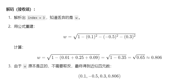
One final improvement. If v is the absolute value of the largest quaternion component, the next largest possible component value occurs when two components have the same absolute value and the other two components are zero. The length of that quaternion (v,v,0,0) is 1, therefore v^2 + v^2 = 1, 2v^2 = 1, v = 1/sqrt(2). This means you can encode the smallest three components in [-0.707107,+0.707107] instead of [-1,+1] giving you more precision with the same number of bits.
With this technique I’ve found that minimum sufficient precision for my simulation is 9 bits per-smallest component. This gives a result of 2 + 9 + 9 + 9 = 29 bits per-orientation (down from 128 bits).
This optimization reduces bandwidth by over 5 megabits per-second, and I think if you look at the right side, you’d be hard pressed to spot any artifacts from the compression.
最后的一个改进。如果 v 是四元数最大分量的绝对值,那么下一个可能的最大分量值出现在两个分量的绝对值相等,另外两个分量为零的情况下。这个四元数的长度为 (v, v, 0, 0),根据四元数的单位长度性质,
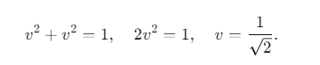
这意味着你可以将最小的三个分量编码在 [-0.707107, +0.707107] 范围内,而不是原来的 [-1, +1] 范围,这样可以在使用相同位数的情况下获得更高的精度。
通过这种技术,我发现对于我的模拟,每个最小分量的最小足够精度是 9 位。这使得每个方向数据的大小为 2 + 9 + 9 + 9 = 29 位(从原来的 128 位减少)。
这项优化减少了超过 5 兆比特每秒(megabits per-second, Mbps) 的带宽,并且如果你观察右侧画面,你很难发现由于压缩而产生的任何视觉伪影(artifacts)。
Optimizing Linear Velocity
What should we optimize next? It’s a tie between linear velocity and position. Both are 96 bits. In my experience position is the harder quantity to compress so let’s start here.
优化线性速度(Optimizing Linear Velocity)
接下来该优化什么?在线性速度(Linear Velocity)和位置(Position)之间,它们都占用了 96 位。根据我的经验,位置通常更难压缩,所以我们先从线性速度入手。
To compress linear velocity we need to bound its x,y,z components in some range so we don’t need to send full float values. I found that a maximum speed of 32 meters per-second is a nice power of two and doesn’t negatively affect the player experience in the cube simulation. Since we’re really only using the linear velocity as a hint to improve interpolation between position sample points we can be pretty rough with compression. 32 distinct values per-meter per-second provides acceptable precision.
为了压缩线性速度(Linear Velocity),我们需要对其 x、y、z 分量 设定一个范围,这样就不需要发送完整的浮点数值。
我发现 最大速度设定为 32 米/秒 是一个不错的选择,它是 2 的幂,并且不会对立方体模拟中的玩家体验产生负面影响。
由于线性速度 只是用于改进位置采样点之间的插值,所以我们可以对其进行较为粗略的压缩。每米每秒 使用 32 个离散值(distinct values) 可以提供足够的精度。
Linear velocity has been bounded and quantized and is now three integers in the range [-1024,1023]. That breaks down as follows: [-32,+31] (6 bits) for integer component and multiply 5 bits fraction precision. I hate messing around with sign bits so I just add 1024 to get the value in range [0,2047] and send that instead. To decode on receive just subtract 1024 to get back to signed integer range before converting to float.
线性速度已被限定范围并量化,现在由三个整数表示,范围为 [−1024,1023]。具体分解如下:整数部分 [−32,+31]使用 6 位表示,小数部分使用 5 位精度。
我不喜欢处理符号位,所以直接加上 1024,使其变为 [0,2047]后再发送。接收时只需减去 1024 恢复为有符号整数范围,然后转换回浮点数即可。
11 bits per-component gives 33 bits total per-linear velocity. Just over 1/3 the original uncompressed size!
We can do even better than this because most cubes are stationary. To take advantage of this we just write a single bit “at rest”. If this bit is 1, then velocity is implicitly zero and is not sent. Otherwise, the compressed velocity follows after the bit (33 bits). Cubes at rest now cost just 127 bits, while cubes that are moving cost one bit more than they previously did: 159 + 1 = 160 bits.
每个分量使用 11 位,总共 33 位 来表示线性速度,仅为原始未压缩大小的 1/3!
我们还能进一步优化,因为大多数立方体是静止的。为了利用这一点,我们添加了一个 “静止”标志位(at rest bit):
-
如果该位为 1,则速度默认为零,不发送任何速度数据。
-
否则,在该位之后发送 压缩后的速度数据(33 位)。
这样,静止的立方体 仅需 127 位,而 运动的立方体 由于额外的 1 位标志位,成本从 159 位增加到 160 位。
假设我们有一个线性速度的分量,例如 12.625 m/s,我们如何用 6 位整数部分 + 5 位小数部分 来表示它呢?
1. 拆分整数和小数部分
原始值:
12.625
-
整数部分:12(范围 [−32,+31],可以用 6 位表示)
-
小数部分:0.6250
2. 小数部分的 5 位量化
小数部分 0.625 需要 量化为 5 位 0.625×32=20
所以 0.625 被表示为 20(5 位二进制:10100)。
最终组合后的 11 位二进制 表示:00110010100
假设接收到 00110010100,拆解:
-
整数部分:
001100= 12 -
小数部分:
10100= 20 -
小数部分还原:
20/32=0.625 -
最终恢复值:
12+0.625=12.625
We can do even better than this because most cubes are stationary. To take advantage of this we just write a single bit “at rest”. If this bit is 1, then velocity is implicitly zero and is not sent. Otherwise, the compressed velocity follows after the bit (33 bits). Cubes at rest now cost just 127 bits, while cubes that are moving cost one bit more than they previously did: 159 + 1 = 160 bits.
我们可以做得更好,因为大多数立方体是静止的。为了利用这一点,我们添加了一个 “静止”标志位”(at rest)。
-
如果该位为 1,则速度默认为零,不发送任何速度数据。
-
否则,该位后面紧跟压缩后的速度数据(33 位)。
这样,静止的立方体 仅需 127 位,而 运动的立方体 由于额外的 1 位标志位,其数据大小从 159 位增加到 160 位。
But why are we sending linear velocity at all? In the previous article we decided to send it because it improved the quality of interpolation at 10 snapshots per-second, but now that we’re sending 60 snapshots per-second is this still necessary? As you can see below the answer is no.
但是,为什么我们还要发送线性速度呢?在上一篇文章中,我们决定发送它,是因为在 每秒 10 个快照(snapshots per-second) 的情况下,它可以提高插值的质量。
但现在我们已经提升到 每秒 60 个快照,它仍然是必要的吗?
如下所示,答案是否定的。
Linear interpolation is good enough at 60HZ. This means we can avoid sending linear velocity entirely. Sometimes the best bandwidth optimizations aren’t about optimizing what you send, they’re about what you don’t send.
在 60HZ 下,线性插值已经足够好。这意味着我们可以完全避免发送线性速度。有时候,最好的带宽优化不是优化你发送的内容,而是优化你不发送的内容。
Optimizing Position
Now we have only position to compress. We’ll use the same trick we used for linear velocity: bound and quantize. I chose a position bound of [-256,255] meters in the horizontal plane (xy) and since in the cube simulation the floor is at z=0, I chose a range of [0,32] meters for z.
现在我们只剩下位置需要压缩。我们将使用与线性速度相同的技巧:限定范围并量化。
我选择了 水平平面(xy)的位置信息范围为 [-256, 255] 米,因为在立方体模拟中,地面位于 z=0,所以我选择了 z 的范围为 [0, 32] 米。
Now we need to work out how much precision is required. With experimentation I found that 512 values per-meter (roughly 2mm precision) provides enough precision. This gives position x and y components in [-131072,+131071] and z components in range [0,16383]. That’s 18 bits for x, 18 bits for y and 14 bits for z giving a total of 50 bits per-position (originally 96).
This reduces our cube state to 80 bits, or just 10 bytes per-cube.
This is approximately 1/4 of the original cost. Definite progress!
Now that we’ve compressed position and orientation we’ve run out of simple optimizations. Any further reduction in precision results in unacceptable artifacts.
现在我们需要计算所需的精度。通过实验,我发现每米 512 个值(大约 2 毫米的精度)提供了足够的精度。这使得 x 和 y 分量 的范围为 [−131072,+131071],z 分量 的范围为 [0,16383]。
这意味着:
-
x 分量需要 18 位
-
y 分量需要 18 位
-
z 分量需要 14 位
总共是 50 位 来表示一个位置(原本是 96 位)。
这将我们的立方体状态压缩到 80 位,即每个立方体 10 字节。
这大约是原始成本的 四分之一。真是一个显著的进展!
现在我们已经压缩了位置和方向,剩下的简单优化方法已经用尽。进一步减少精度会导致无法接受的伪影(artifacts)
Delta Compression
Can we optimize further? The answer is yes, but only if we embrace a completely new technique: delta compression.
还能进一步优化吗?答案是 可以,但前提是我们采用一种全新的技术:增量压缩(Delta Compression)。
Delta compression sounds mysterious. Magical. Hard. Actually, it’s not hard at all. Here’s how it works: the left side sends packets to the right like this: “This is snapshot 110 encoded relative to snapshot 100”. The snapshot being encoded relative to is called the baseline. How you do this encoding is up to you, there are many fancy tricks, but the basic, big order of magnitude win comes when you say: “Cube n in snapshot 110 is the same as the baseline. One bit: Not changed!”
增量压缩听起来神秘、魔幻、难以理解。实际上,它一点也不难。它的工作原理是这样的:左侧发送数据包到右侧,内容是:“这是相对于快照 100 编码的快照 110”。被用作编码基准的快照称为 基准快照(baseline)。如何进行这种编码取决于你,有很多复杂的技巧,但基本的、最显著的提升来自于你可以说:“快照 110 中的立方体 n 与基准快照相同。一个位:未改变!”
To implement delta encoding it is of course essential that the sender only encodes snapshots relative to baselines that the other side has received, otherwise they cannot decode the snapshot. Therefore, to handle packet loss the receiver has to continually send “ack” packets back to the sender saying: “the most recent snapshot I have received is snapshot n”. The sender takes this most recent ack and if it is more recent than the previous ack updates the baseline snapshot to this value. The next time a packet is sent out the snapshot is encoded relative to this more recent baseline. This process happens continuously such that the steady state becomes the sender encoding snapshots relative to a baseline that is roughly RTT (round trip time) in the past.
要实现增量编码,当然必须确保发送方只对接收方已经收到的基准快照进行编码,否则接收方无法解码该快照。因此,为了处理数据包丢失,接收方必须不断地向发送方发送 “确认(ack)” 数据包,告诉发送方:“我接收到的最新快照是快照 n”。发送方接收到这个最新的确认后,如果它比之前的确认更新,就将基准快照更新为这个值。下次发送数据包时,快照将相对于这个更新后的基准快照进行编码。这个过程会持续进行,直到达到稳定状态,发送方将快照相对于大约 RTT(往返时间) 前的基准快照进行编码。
There is one slight wrinkle: for one round trip time past initial connection the sender doesn’t have any baseline to encode against because it hasn’t received an ack from the receiver yet. I handle this by adding a single flag to the packet that says: “this snapshot is encoded relative to the initial state of the simulation” which is known on both sides. Another option if the receiver doesn’t know the initial state is to send down the initial state using a non-delta encoded path, eg. as one large data block, and once that data block has been received delta encoded snapshots are sent first relative to the initial baseline in the data block, then eventually converge to the steady state of baselines at RTT.
有一个小问题:在初始连接后的一个往返时间内,发送方没有基准快照可供编码,因为它还没有收到接收方的确认。为了解决这个问题,我在数据包中添加了一个标志位,表示:“这个快照是相对于模拟的初始状态进行编码的”,这个初始状态在双方都是已知的。另一个选择是,如果接收方不知道初始状态,可以通过非增量编码的方式发送初始状态,例如作为一个大的数据块,等到该数据块被接收后,增量编码的快照将首先相对于数据块中的初始基准进行编码,然后最终与基准快照在往返时间(RTT)内达到稳定状态。
As you can see above this is a big win. We can refine this approach and lock in more gains but we’re not going to get another order of magnitude improvement past this point. From now on we’re going to have to work pretty hard to get a number of small, cumulative gains to reach our goal of 256 kilobits per-second.
如上所示,这是一个很大的进步。我们可以优化这个方法并锁定更多的收益,但我们无法在这一点上获得另一个数量级的提升。从现在开始,我们必须付出相当大的努力,通过一系列小的、累积的优化,才能实现每秒 256 千比特的目标。
Incremental Improvements
First small improvement. Each cube that isn’t sent costs 1 bit (not changed). There are 901 cubes so we send 901 bits in each packet even if no cubes have changed. At 60 packets per-second this adds up to 54kbps of bandwidth. Seeing as there are usually significantly less than 901 changed cubes per-snapshot in the common case, we can reduce bandwidth by sending only changed cubes with a cube index [0,900] identifying which cube it is. To do this we need to add a 10 bit index per-cube to identify it.
增量改进
第一个小改进:每个未发送的立方体都需要 1 位(未改变)。总共有 901 个立方体,因此即使没有立方体发生变化,每个数据包也会发送 901 位。以每秒 60 个数据包计算,这相当于 54kbps 的带宽。考虑到在大多数情况下,每个快照中发生变化的立方体通常远少于 901 个,我们可以通过只发送发生变化的立方体来减少带宽,并使用立方体索引 [0,900] 来标识它是哪个立方体。为了实现这一点,我们需要为每个立方体添加一个 10 位的索引来标识它。
There is a cross-over point where it is actually more expensive to send indices than not-changed bits. With 10 bit indices, the cost of indexing is 10*n bits. Therefore it’s more efficient to use indices if we are sending 90 cubes or less (900 bits). We can evaluate this per-snapshot and send a single bit in the header indicating which encoding we are using: 0 = indexing, 1 = changed bits. This way we can use the most efficient encoding for the number of changed cubes in the snapshot.
This reduces the steady state bandwidth when all objects are stationary to around 15 kilobits per-second. This bandwidth is composed entirely of our own packet header (uint16 sequence, uint16 base, bool initial) plus IP and UDP headers (28 bytes).
当所有物体都处于静止状态时,这将把稳定状态的带宽减少到大约 15 kilobits per-second。这个带宽完全由我们自己的数据包头部(uint16 序列号、uint16 基准、bool 初始标志)以及 IP 和 UDP 头部(28 字节)组成。
Next small gain. What if we encoded the cube index relative to the previous cube index? Since we are iterating across and sending changed cube indices in-order: cube 0, cube 10, cube 11, 50, 52, 55 and so on we could easily encode the 2nd and remaining cube indices relative to the previous changed index, e.g.: +10, +1, +39, +2, +3. If we are smart about how we encode this index offset we should be able to, on average, represent a cube index with less than 10 bits.
下一个小的优化。假设我们将立方体索引相对于前一个立方体索引进行编码会怎样?由于我们是按顺序迭代并发送变化的立方体索引:立方体 0、立方体 10、立方体 11、50、52、55 等,我们可以轻松地将第二个及后续的立方体索引相对于前一个变化的索引进行编码,例如:+10、+1、+39、+2、+3。如果我们聪明地处理这个索引偏移的编码,我们应该能够平均使用少于 10 bits来表示一个立方体索引。
例如:
-
第一个立方体是 0,我们直接发送它。
-
第二个立方体是 10,它与第一个立方体的索引差是 +10,我们只需要发送 10(相对差值)。
-
第三个立方体是 11,它与第二个立方体的索引差是 +1,我们只需要发送 1(相对差值)。
-
第四个立方体是 50,它与第三个立方体的索引差是 +39,我们只需要发送 39(相对差值)。
-
第五个立方体是 52,它与第四个立方体的索引差是 +2,我们只需要发送 2(相对差值)。
-
第六个立方体是 55,它与第五个立方体的索引差是 +3,我们只需要发送 3(相对差值)。
通过这种方式,我们只需要发送每个变化的 差值,而不是每个立方体的完整索引。这样,后续的差值通常会比原始索引小得多,从而节省了大量的带宽。
为什么这能节省带宽?
因为如果我们直接发送立方体的完整索引,每个索引可能需要 10 位,而如果我们发送相对差值,由于差值通常很小,可以使用更少的位。例如,如果差值在 0 到 100 之间,我们可以使用 7 位来表示这个差值,比直接发送完整的 10 位索引要节省带宽。
The best encoding depends on the set of objects you interact with. If you spend a lot of time moving horizontally while blowing cubes from the initial cube grid then you hit lots of +1s. If you move vertically from initial state you hit lots of +30s (sqrt(900)). What we need then is a general purpose encoding capable of representing statistically common index offsets with less bits.
最佳的编码方式取决于你与哪些物体交互。如果你花很多时间在水平移动,并且从初始立方体网格中吹出立方体,那么你会遇到很多 +1 的差值。如果你从初始状态垂直移动,则会遇到很多 +30 的差值(sqrt(900))。因此,我们需要一种通用的编码方式,能够用更少的位表示统计上常见的索引偏移。
After a small amount of experimentation I came up with this simple encoding:
- [1,8] => 1 + 3 (4 bits)
- [9,40] => 1 + 1 + 5 (7 bits)
- [41,900] => 1 + 1 + 10 (12 bits)
Notice how large relative offsets are actually more expensive than 10 bits. It’s a statistical game. The bet is that we’re going to get a much larger number of small offsets so that the win there cancels out the increased cost of large offsets. It works. With this encoding I was able to get an average of 5.5 bits per-relative index.
请注意,较大的相对偏移实际上比 10 位的成本更高。这是一个统计学上的博弈。我们的假设是,绝大多数情况下我们会遇到较小的偏移,这样小偏移带来的节省将抵消大偏移带来的成本增加。它是有效的。通过这种编码,我能够将每个相对索引的平均位数降低到 5.5 位。
Now we have a slight problem. We can no longer easily determine whether changed bits or relative indices are the best encoding. The solution I used is to run through a mock encoding of all changed cubes on packet write and count the number of bits required to encode relative indices. If the number of bits required is larger than 901, fallback to changed bits.
Here is where we are so far, which is a significant improvement:
现在我们遇到了一个小问题。我们不再能轻松地判断是使用变化的位还是相对索引作为最佳编码方式。我的解决方案是在数据包写入时,先模拟对所有变化的立方体进行编码,并计算使用相对索引编码所需的位数。如果所需的位数超过 901,则回退到使用变化的位编码。
到目前为止,我们已经取得了显著的改进:
https://gafferongames.com/videos/snapshot_compression_delta_relative_index.mp4
Next small improvement. Encoding position relative to (offset from) the baseline position. Here there are a lot of different options. You can just do the obvious thing, eg. 1 bit relative position, and then say 8-10 bits per-component if all components have deltas within the range provided by those bits, otherwise send the absolute position (50 bits).
下一个小的优化。将位置相对于基准位置进行编码(即偏移量)。这里有很多不同的选择。你可以做最简单的事情,例如使用 1 位表示相对位置,然后如果所有组件的增量都在这些位提供的范围内,就使用每个组件 8-10 位,如果不在该范围内,则发送绝对位置(50 位)。
This gives a decent encoding but we can do better. If you think about it then there will be situations where one position component is large but the others are small. It would be nice if we could take advantage of this and send these small components using less bits.
这提供了一个不错的编码方式,但我们可以做得更好。如果你仔细想想,就会发现有些情况其中一个位置组件很大,而其他组件很小。如果我们能够利用这一点,使用更少的位来发送这些小的组件,那将会更好。
It’s a statistical game and the best selection of small and large ranges per-component depend on the data set. I couldn’t really tell looking at a noisy bandwidth meter if I was making any gains so I captured the position vs. position base data set and wrote it to a text file for analysis.
这实际上是一个统计问题,每个组件的小范围和大范围的最佳选择取决于数据集。由于看着一个嘈杂的带宽计很难判断是否取得了任何进展,我捕获了位置与基准位置的数据集,并将其写入文本文件进行分析。
I wrote a short ruby script to find the best encoding with a greedy search. The best bit-packed encoding I found for the data set works like this: 1 bit small per delta component followed by 5 bits if small [-16,+15] range, otherwise the delta component is in [-256,+255] range and is sent with 9 bits. If any component delta values are outside the large range, fallback to absolute position. Using this encoding I was able to obtain on average 26.1 bits for changed positions values.
我写了一个简短的 Ruby 脚本来通过贪婪搜索找到最佳编码。我为数据集找到的最佳位压缩编码方式如下:每个增量组件使用 1 位表示是否为小范围,然后如果增量在 [-16, +15] 范围内,使用 5 位表示;否则,如果增量在 [-256, +255] 范围内,则使用 9 位表示。如果任何组件的增量值超出了大范围,则回退到绝对位置。使用这种编码方式,我能够将更改的位置值的平均位数压缩到 26.1 位。
Delta Encoding Smallest Three
Next I figured that relative orientation would be a similar easy big win. Problem is that unlike position where the range of the position offset is quite small relative to the total position space, the change in orientation in 100ms is a much larger percentage of total quaternion space.
接下来我想到了相对方向可能也会带来类似的巨大优化。问题是,与位置不同,位置偏移的范围相对总位置空间来说是比较小的,而在 100 毫秒内,方向的变化占总四元数空间的比例要大得多。
I tried a bunch of stuff without good results. I tried encoding the 4D vector of the delta orientation directly and recomposing the largest component post delta using the same trick as smallest 3. I tried calculating the relative quaternion between orientation and base orientation, and since I knew that w would be large for this (rotation relative to identity) I could avoid sending 2 bits to identify the largest component, but in turn would need to send one bit for the sign of w because I don’t want to negate the quaternion. The best compression I could find using this scheme was only 90% of the smallest three. Not very good.
我尝试了很多方法,但都没有得到好的结果。我尝试直接编码增量方向的 4D 向量,并使用与smallest 3相同的技巧,在增量后重组最大的分量。我也尝试计算方向与基准方向之间的相对四元数,并且由于我知道 w 在这种情况下会很大(相对于单位矩阵的旋转),我可以避免发送 2 位来标识最大的分量,但反过来,我需要发送一个位来表示 w 的符号,因为我不想反转四元数。使用这种方案,我能找到的最佳压缩率仅为 smallest three的 90%。效果不太好。
I was about to give up but I run some analysis over the smallest three representation. I found that 90% of orientations in the smallest three format had the same largest component index as their base orientation 100ms ago. This meant that it could be profitable to delta encode the smallest three format directly. What’s more I found that there would be no additional precision loss with this method when reconstructing the orientation from its base. I exported the quaternion values from a typical run as a data set in smallest three format and got to work trying the same multi-level small/large range per-component greedy search that I used for position.
我差点放弃了,但我对 smallest three表示进行了分析。我发现,在 smallest three格式中,90%的方向与它们在 100 毫秒前的基准方向具有相同的最大分量索引。这意味着直接对 smallest three 格式进行增量编码可能是有利的。更重要的是,我发现使用这种方法重建方向时不会有额外的精度损失。我将一个典型运行中的四元数值导出为 smallest three格式的数据集,并开始尝试使用我在位置编码中使用的相同的多级小/大范围每个分量贪婪搜索。
The best encoding found was: 5-8, meaning [-16,+15] small and [-128,+127] large. One final thing: as with position the large range can be extended a bit further by knowing that if the component value is not small the value cannot be in the [-16,+15] range. I leave the calculation of how to do this as an exercise for the reader. Be careful not to collapse two values onto zero.
我找到的最佳编码是:5-8,意味着[-16,+15]的小范围和[-128,+127]的大范围。最后一件事:与位置相同,知道如果分量值不小,那么该值就不可能在[-16,+15]范围内,可以稍微扩展大范围。如何做这个计算留给读者作为练习。需要小心不要将两个值压缩为零。
The end result is an average of 23.3 bits per-relative quaternion. That’s 80.3% of the absolute smallest three.
That’s just about it but there is one small win left. Doing one final analysis pass over the position and orientation data sets I noticed that 5% of positions are unchanged from the base position after being quantized to 0.5mm resolution, and 5% of orientations in smallest three format are also unchanged from base.
These two probabilities are mutually exclusive, because if both are the same then the cube would be unchanged and therefore not sent, meaning a small statistical win exists for 10% of cube state if we send one bit for position changing, and one bit for orientation changing. Yes, 90% of cubes have 2 bits overhead added, but the 10% of cubes that save 20+ bits by sending 2 bits instead of 23.3 bit orientation or 26.1 bits position make up for that providing a small overall win of roughly 2 bits per-cube.
最终结果是平均每个相对四元数使用了23.3位。这是绝对最小三表示的80.3%。
差不多就到这里,但还有一个小的优化。在对位置和方向数据集进行最后一次分析时,我注意到在量化到0.5mm分辨率后,有5%的位置与基准位置相同,另外5%的最小三格式的方向也与基准方向相同。
这两个概率是互斥的,因为如果两个都相同,那么立方体将保持不变,因此不会发送。这意味着在10%的立方体状态中,如果我们发送一个表示位置变化的位和一个表示方向变化的位,就可以获得一个小的统计优势。是的,90%的立方体会增加2个位的开销,但对于那10%的立方体,通过发送2个位而不是23.3位的方向或26.1位的位置节省了20多个位,因此能够弥补这种开销,提供一个约为2个位的整体小幅优化。
Conclusion
And that’s about as far as I can take it using traditional hand-rolled bit-packing techniques. You can find source code for my implementation of all compression techniques mentioned in this article here.
It’s possible to get even better compression using a different approach. Bit-packing is inefficient because not all bit values have equal probability of 0 vs 1. No matter how hard you tune your bit-packer a context aware arithmetic encoding can beat your result by more accurately modeling the probability of values that occur in your data set. This implementation by Fabian Giesen beat my best bit-packed result by 25%.
It’s also possible to get a much better result for delta encoded orientations using the previous baseline orientation values to estimate angular velocity and predict future orientations rather than delta encoding the smallest three representation directly.
结论
这就是我使用传统的手工位打包技术所能达到的极限。你可以在这里找到我实现的所有压缩技术的源代码。
通过不同的方法,实际上可以获得更好的压缩效果。位打包之所以低效,是因为并非所有位值的0和1出现的概率相等。无论你如何调整位打包器,基于上下文的算术编码都能通过更准确地建模数据集中出现值的概率,超越你的结果。Fabian Giesen的实现就比我最好的位打包结果提高了25%。
对于增量编码的方向,使用先前的基准方向值来估计角速度,并预测未来的方向,而不是直接增量编码最小三表示,这也能获得更好的结果。

 浙公网安备 33010602011771号