Node2Vec、Word2Vec中Skip Gram的超详细解析

概述

自然语言作为人类意义传递的复杂符号系统，其基本表义单元是离散的词汇元素。词向量 $Word Vector$ 作为词汇的数学表征形式，本质上是将词语映射至实数域的高维向量空间，也称词嵌入 $Word Embedding$ 。该技术通过连续稠密向量刻画词语的语义和语法特征，已成为当代自然语言处理任务的重要基础方法。

~wordembedding

由于任何语言的词汇量都极为庞大，且丰富的语义与上下文关系无法通过人工标注完全覆盖，因此依赖于海量文本的无/自监督学习技术成为学习词汇分布式表示的核心手段。其中， $Word2Vec$ 作为词嵌入领域的经典自监督学习方法具有重要意义和价值。

语言序列固有的时序性要求词向量建模需符合语序约束。从概率视角分析，理想的语言模型应当最大化语句序列的联合概率，该概率可分解为顺序条件概率的连乘形式：

\[P(w_1, w_2, \cdots, w_T) = \prod_{t=1}^{T} P(w_t \mid w_1, \cdots, w_{t-1}) \]

这种全序列建模面临计算难题：随着序列长度增加，条件概率估计所需参数量累计增长。

为突破计算瓶颈，$Word2Vec$ 引入滑动窗口约束建模范围。设窗口半径为 $w$ ，对中心词wt的预测仅依赖其固定窗口内的上下文单词：

\[P(w_t∣w_{t−w},⋯,w_{t−1},w_{t+1},⋯,w_{t+w}) \]

这种局部建模策略将联合概率分解转化为有限窗口内的条件概率乘积，显著降低模型复杂度，实现了计算可行性。基于这种建模方法，$Word2Vec$ 提出了两种高效方法：

~word2vec

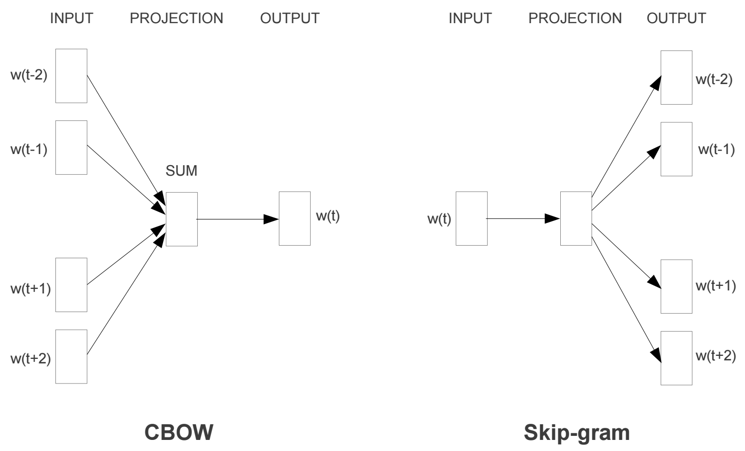
连续词袋模型 $CBOW$ ：通过上下文窗口词预测中心词。
跳字模型 $Skip-gram$ ：根据给定的中心词预测上下文窗口内词。

实际上，以上任务训练模型的真正目的是获得模型基于训练数据学得的隐层权重作为词嵌入的向量表示。为了得到这些权重，首先构建完整的神经网络作为 $fake$ $task$ ，之后再通过训练好的神经网络间接地得到词向量矩阵。当模型通过大量语料训练完成词汇预测任务时，网络隐层权重自发形成词向量的稠密低维表示，这种间接学习方法将词向量获取转化为参数优化过程的副产品。

$Skip$ $Gram$ 模型

模型概述

$Skip$ $Gram$ 模型是一种浅层神经网络架构，具有输入层、隐藏层以及输出层，每个层承担特定计算任务。

输入层接收目标词的 $one$-$hot$ 编码向量表示，向量维度等于词汇表大小，与目标词对应的索引位置设为 $1$，其余为 $0$ 。随后输入向量与隐藏层的权重矩阵进行点积运算，产生一个低维稠密向量，即隐含的词嵌入表示；

隐藏层不采用任何激活函数，使得计算为单纯的线性变换。

输出层进一步处理隐藏层的输出向量：通过将其与另一个权重矩阵执行点积，获得每个潜在上下文词的得分向量。得分向量最终被馈送至 $softmax$ 激活函数，计算出归一化的概率分布向量，向量元素总和为 $1$ ，概率分布表示每个词汇项出现在目标词固定上下文窗口内的相对概率。

余弦相似度

构建单词嵌入后，可以使用 $Cosine$ $Similarity$ 指标从词汇表中输入单词来查找相似或相关的单词，进而测试它们。

余弦相似度通过计算两个向量之间夹角的余弦来表示两个向量方向上的相似性。其值范围从 $-1$ 到 $1$，其中 $1$ 表示方向相同（它们之间的 $0°$ 角），$0$ 表示正交向量（它们之间的 $90°$ 角），-1 指向截然相反的向量（它们之间的 $180°$ 角）:

~CosineSimilarity

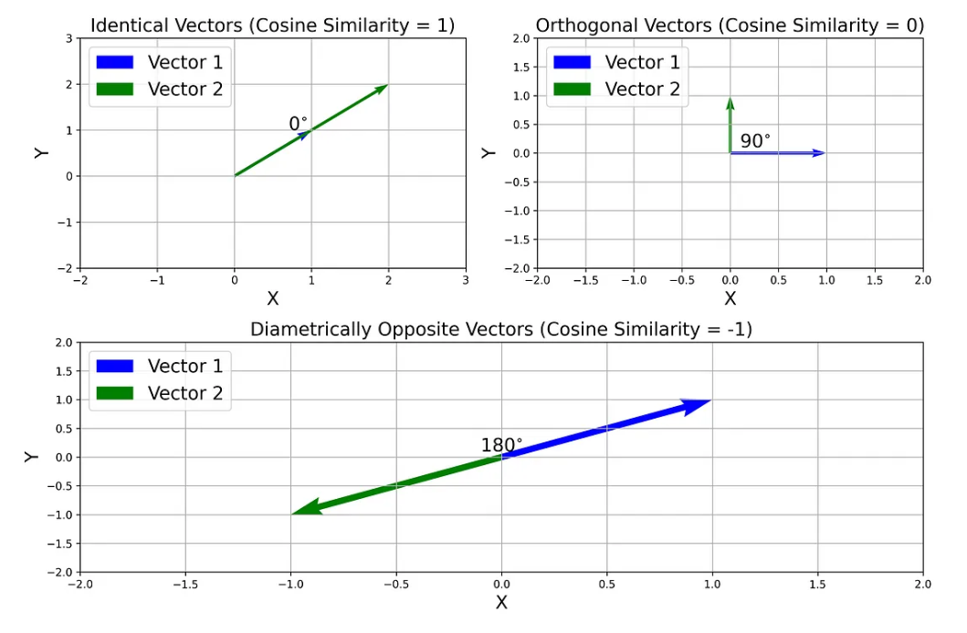
就词嵌入向量而言，余弦相似度 $1$ 表示词语高度相关或相似（如 $happy$ 和 $content$），0 表示词语不相关或不相似（如 $car$ 和 $apple$），$-1$ 表示词语高度不相关或极不相似（如 $good$ 和 $bad$）。

两个向量 $a$ 和 $b$ 之间的余弦相似度为：

\[\text{cosine similarity}=\frac{\mathrm{a}\cdot\mathrm{b}}{\|\mathrm{a}\|\|\mathrm{b}\|} \]

为了查找与特定单词相似或相关的单词，可以计算其嵌入向量与单词嵌入矩阵中所有其他向量之间的余弦相似度。

语料库 $Corpus$

语料库使训练模型的数据集合，用来帮助模型学习词语间的语义关联模式。在图嵌入过程中，使用随机游走方法采样得到的随机游走序列作为等同于 $Word$ $Embedding$ 使用的语料库中的句子。

假设存在一个从该语料库抽取的词汇表 $vocabulary$ ，其中包含十个单词：
graph、is、a、good、way、to、visualize、data、very、at
基于 $vocabulary$ ，可以构建出结构完整且语义清晰的句子实例：

Graph is a good way to visualize data.

滑动窗口采样

$Skip$ $Gram$ 模型采用滑动窗口采样技术来生成训练样本。该方法使用一个$Sliding$ $Window$ ，在句子中的每个单词中按顺序移动，在一定范围内目标词与它前后的每个上下文词组合。

以下window_size=1:

~window_sampling

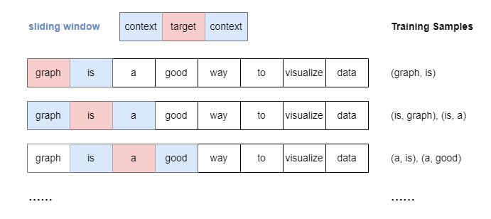
当window_size>1时，则无论上下文单词与目标单词的距离如何，都会平等地处理位于指定窗口内的所有上下文单词形成单词对。

$One$-$hot$ 编码

由于单词无法被机器学习模型直接处理，我们必须将其转化为可机识别的表示形式，常用方法是使用 $One$-$hot$ 编码，该方法通过将每个词表示为唯一的二值向量来实现，编码向量的维度与词汇表大小相同，仅有一个元素的值为 $1$ ，该元素的位置对应词在词汇表中的索引序号，其余元素均为 $0$ 。

以先前提供的包含 10 个词语的词汇表为例，其中每个词均具有专属的 $One$-$hot$ 编码向量表示:

Word	One-hot 编码
graph	1000000000
is	0100000000
a	0010000000
good	0001000000
way	0000100000
to	0000010000
visualize	0000001000
data	0000000100
very	0000000010
at	0000000010

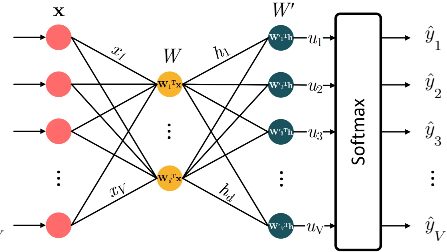
$Skip$-$gram$ 架构

~skipgram01

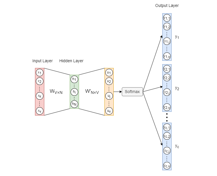
$Skip$-$gram$ 模型的架构如上图所示，其中：

输入向量xV×1是目标单词的 $One$-$hot$ 编码，并且 $V$ 是词汇表中的单词数。
$W_{V×N}$ 是 $input→hidden$ 权重矩阵，而 $N$ 是单词嵌入的维度。
$h_{N×1}$ 是隐藏层向量。
$W^′_{N×V}$是 $hidden→output$ 权重矩阵。$W^′$ 和 $W$ 是不同的，$W^′$ 不是 $W$ 。
$u_{V×1}$ 是应用激活函数 $Softmax$ 之前的向量。
输出向量 $y_c(c=1,2,...,C)$ 称为 $panels$ ，对应目标单词 $C$ 的上下文词。

$Softmax$：$Softmax$ 函数作为激活函数，用于将数值向量归一化为概率分布向量。在这个变换的向量中所有概率的总和等于 $1$ 。$Softmax$ 的公式：

\[Softmax(u_j)=\frac{e^{u_j}}{\sum_ie^{u_i}} \]

在上述 $Skip$-$gram$ 模型中：

从输入层到隐藏层的连接在形式上为全连接，权重由 $V×N$ 权重矩阵 $W$ 定义。

理论上层次间存在 $V×N$ 个连接（每个输入神经元到每个投影神经元），但每次计算时，由于 $One$-$hot$ 输入的稀疏性，仅有一个输入神经元激活（值为 $1$ ）只有该神经元对应的 $N$ 个连接有效，其余 $(V−1)×N$ 个连接的权重不参与计算。

从隐藏层到输出层的连接是严格的全连接，权重由 $N×V$ 权重矩阵 $W^′$ 定义。

每个隐藏层神经元到每个输出层神经元之间都存在连接，输出层的 $C$ 个 $panels$ 共享相同的连接权重 $W^′$ ，每次计算时所有 $N×V$ 个连接都参与计算，通过矩阵乘法 $h\cdot W^′$ 同时计算所有输出值。

前向传播

在示例中，$V=10$，设置 $N=2$ （即隐层神经元节点数），随机初始化权重矩阵 $W^′$ 和 $W$ 如下所示。然后，使用样本 $(is, graph)$， $(is, a)$ ：
~Forward_Propagation

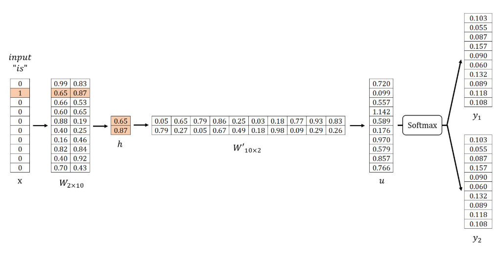
$Input Layer → Hidden Layer$

获取隐藏层向量 $h$ 的方法： $$u=hW^{\prime T}$$给定 $x$ 是一个独热编码向量（仅 $xₖ = 1$），则 $h$ 对应于矩阵 $W$ 的第 $k$ 行。该操作本质上是简单的向量查找过程：

\[h=v_{wI}^T \]

其中 $v_{wI}$ 是目标词的输入向量，矩阵 $W$ 的每一行（记为 $v_w$）是词汇表中每个词的最终嵌入表示。

$Hidden Layer → Output Layer$

获取向量 $u$ 的方法：

\[u=hW^{\prime T} \]

向量 $u$ 的第 $j$ 个分量等于向量 $h$ 与矩阵 $W'$ 第 $j$ 列向量转置的点积： $$u_j=h\cdot{v_{w_j}^{\prime}}T$$其中 $v_{w_j}^{\prime}$ 是词汇表 $vocabulary$ 中第 $j$ 个词的输出向量。

[!注意]
在 $Skip$-$gram$ 模型的设计中，词汇表中的每个词都具有两种不同的向量表示：输入向量 $v_w$ 和输出向量 $v_{w}^{\prime}$ ，当词语作为目标词时采用输入向量表示，而作为上下文词时则采用输出向量表示。

在计算过程中，$u_j$ 本质上体现了目标词输入向量 $v_{wI}$ 与第 $j$ 个词输出向量 $v_{w_j}^{\prime}$ 的点积关系，两个向量间的相似度越高，其点积结果越大。

最终被用作词嵌入的实际是输入向量。这种对输入/输出向量的分离机制，有效优化了计算过程，提升了模型训练与推理的效率和准确性。

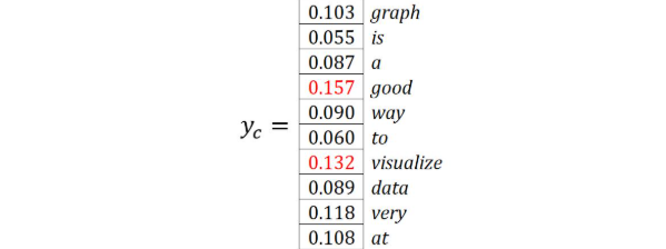
通过以下公式计算输出 $y_C$：

\[y_{c}=Softmax(u)，y_{c,j}=\frac{e^{u_j}}{\sum_{i=1}^Ve^{u_i}} \]

其中 $y_{c,j}$ 是向量 $y_c$ 的第 $j$ 个分量，表示在给定目标词条件下，预测词表中第 $j$ 个词作为上下文词的条件概率，显然所有概率之和为 $1$ 。

概率值最高的 $C$ 个词被视为预测的上下文词，在示例中，设定 $C=2$ ，预测的上下文词是 good 和 visualize 。

~y_c

反向传播

权重更新机制

使用随机梯度下降 $SGD$  对权重矩阵 $W$ 和 $W^′$ 进行反向传播更新。

损失函数定义

最大化 $C$ 个上下文词的出现概率，即最大化概率乘积：

\[max\prod_{c=1}^c\frac{e^{u_{j_c^*}}}{\sum_{i=1}^Ve^{u_i}} \]

其中 $j_c^∗$ 表示第 $c$ 个目标上下文词在词表中的索引，由于最小化通常被认为比最大化更直接、更实用，因此对上述目标进行一些转换：

\[\begin{aligned}max\prod_{c=1}^{C}\frac{e^{u_{j_{c}^{*}}}}{\sum_{i=1}^{\nu}e^{u_{i}}}&=min\left(-log\prod_{c=1}^{C}\frac{e^{u_{j_{c}^{*}}}}{\sum_{i=1}^{V}e^{u_{i}}}\right)\\&=min\left(-\sum_{c=1}^{C}log\frac{e^{u_{j_{c}^{*}}}}{\sum_{i=1}^{V}e^{u_{i}}}\right)=min\left(-\sum_{c=1}^{C}u_{j_{c}^{*}}-log\sum_{i=1}^{V}e^{u_{i}}\right)\\&=min(-\sum_{c=1}^{C}u_{j_{c}^{*}}+C\cdot log\sum_{i=1}^{V}e^{u_{i}})\end{aligned} \]

因此，损失函数 $E$ 表示为：

\[E=-\sum_{c=1}^cu_{j_c^*}+C\cdot log\sum_{i=1}^Ve^{u_i} \]

对 $E$ 求关于 $u_j$ 的偏导数：

\[\begin{aligned}\frac{\partial E}{\partial u_{j}}&=\frac{\partial}{\partial u_{j}}\left(-\sum_{c=1}^{c}u_{j_{c}^{*}}+C\cdot log\sum_{i=1}^{V}e^{u_{i}}\right)=C\cdot\frac{\partial}{\partial u_{j}}log\sum_{i=1}^{V}e^{u_{i}}-\sum_{c=1}^{C}\frac{\partial u_{j_{c}^{*}}}{\partial u_{j}}\\&=C\cdot\frac{1}{\sum_{i=1}^{V}e^{u_{i}}}\cdot\frac{\partial e^{u_{j}}}{\partial u_{j}}-\sum_{c=1}^{C}\frac{\partial u_{j_{c}^{*}}}{\partial u_{j}}=C\cdot\frac{e^{u_{j}}}{\sum_{i=1}^{V}e^{u_{i}}}-\sum_{c=1}^{C}\frac{\partial u_{j_{c}^{*}}}{\partial u_{j}}\\&=\sum_{c=1}^{c}\left(y_{c,j}-\frac{\partial u_{j}^{*}}{\partial u_{j}}\right)=\begin{cases}\sum_{c=1}^{C}\left(y_{c,j}-1\right),j=j_{c}^{*}\\\sum_{c=1}^{C}\left(y_{c,j}-0\right),j\neq j_{c}^{*}&\end{cases}\end{aligned} \]

引入简化符号（$t_c$ 为第 $c$ 个上下文词的独热编码向量）：

\[e_{c,j}=\begin{cases}y_{c,j}-1,j=j_c^*\\y_{c,j}-0,j\neq j_c^*&\end{cases}=y_{c,j}-t_{c,j} \]

示例中，$t_1$ 和 $t_2$ 是单词 Graph 和 a 的 $one$-$hot$ 编码向量，因此 $e_1$ 和 $e_2$ 为：
~e_1
~e_2
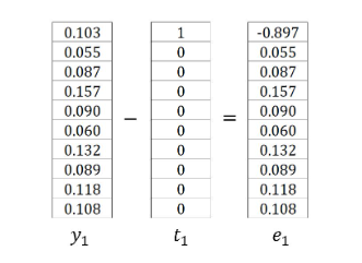
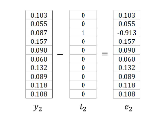
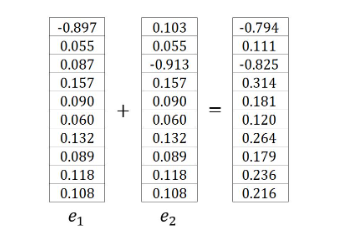
因此 $∂E/∂u_j$ 可以写成：

\[\frac{\partial E}{\partial u_j}=\sum_{c=1}^ce_{c,j} \]

~e1_+e2

$Output Layer → Hidden Layer$

对矩阵 $W^′$ 中的所有权重进行调整，更新所有词的输出向量，计算损失函数 $E$ 对 $w_{ij}^′$ 的偏导数：

\[\frac{\partial E}{\partial w_{ij}^{\prime}}=\frac{\partial E}{\partial u_{j}}\cdot\frac{\partial u_{j}}{\partial w_{ij}^{\prime}}=\frac{\partial E}{\partial u_{j}}\cdot\frac{\partial}{\partial w_{ij}^{\prime}}(h_{1}w_{1j}^{\prime}+\cdots+h_{i}w_{ij}^{\prime}+\cdots+h_{V}w_{Vj}^{\prime})=\sum_{c=1}^{C}e_{c,j}\cdot h_{i} \]

根据学习率 $η$ 调整 $w_{ij}^′$：

\[w_{ij}^{\prime}:=w_{ij}^{\prime}-\eta\cdot\sum_{c=1}^Ce_{c,j}\cdot h_i \]

设 $η=0.4$，例如 $w_{14}^′=0.86$ 和 $w_{24}^′=0.67$ 更新为：

\[w_{14}^{^{\prime}}=w_{14}^{^{\prime}}-\eta\cdot(e_{1,4}+e_{2,4})\cdot h_{1}=0.86-0.4\times0.314\times0.65=0.78 \]

\[w_{24}^{^{\prime}}=w_{24}^{^{\prime}}-\eta\cdot(e_{1,4}+e_{2,4})\cdot h_{2}=0.67-0.4\times0.314\times0.87=0.56 \]

$Hidden Layer → Input Layer$

调整矩阵 W 中与目标词输入向量对应的权重，隐藏向量 $h$ 通过提取 $W$ 的第 $k$ 行获得（给定 $x_k=1$）：

\[h_{i}=w_{ki} \]

计算损失函数 $E$ 对 $w_{ki}$ 的偏导数：

\[\begin{aligned}\frac{\partial E}{\partial w_{ki}}&=\frac{\partial E}{\partial h_{i}}\cdot\frac{\partial h_{i}}{\partial w_{ki}}=\sum_{j=1}^{V}\left(\frac{\partial E}{\partial u_{j}}\cdot\frac{\partial u_{j}}{\partial h_{i}}\right)\cdot\frac{\partial h_{i}}{\partial w_{ki}}\\&=\sum_{j=1}^{V}\left(\frac{\partial E}{\partial u_{j}}\cdot\left(\frac{\partial}{\partial h_{i}}\sum_{i=1}^{N}h_{i}\cdot w_{ij}^{\prime}\right)\right)\cdot\frac{\partial}{\partial w_{ki}}w_{ki}\\&=\sum_{j=1}^{V}\left(\frac{\partial E}{\partial u_{j}}\cdot w_{ij}^{\prime}\right)\cdot1=\sum_{j=1}^{V}\sum_{c=1}^{c}e_{c,j}\cdot w_{ij}^{\prime}\end{aligned} \]

根据学习率 $η$ 调整 $w_{ki}$：

\[w_{ki}:=w_{ki}-\eta\cdot\sum_{j=1}^{V}\sum_{c=1}^{C}e_{c,j}\cdot w_{ij}^{\prime} \]

示例中，$k=2$，因此 $w_{21}=0.65$ 和 $w_{22}=0.87$ 更新为：

\[\frac{\partial E}{\partial w_{2,1}}=(e_{1,1}+e_{2,1})\cdot w_{11}^{^{\prime}}+(e_{1,2}+e_{2,2})\cdot w_{12}^{^{\prime}}+...+(e_{1,10}+e_{2,10})\cdot w_{1,10}^{^{\prime}}=0.283 \]

\[w_{21}=w_{21}\cdot\eta\cdot\frac{\partial E}{\partial w_{21}}=0.65-0.4\times0.283=0.54 \]

\[\frac{\partial E}{\partial w_{22}}=(e_{1,1}+e_{2,1})\cdot w_{21}^{^{\prime}}+(e_{1,2}+e_{2,2})\cdot w_{22}^{^{\prime}}+...+(e_{1,10}+e_{2,10})\cdot w_{2,10}^{^{\prime}}=0.081 \]

\[w_{22}=w_{22}-\eta\cdot\frac{dE}{\partial w_{22}}=0.87-0.4\times0.081=0.84 \]

$Skip$-$gram$ 优化

由于各种计算需求，基本的 $Skip$-$gram$ 模型几乎无法使用。

矩阵的大小 $W$ 和 $W^′$ 取决于词汇表大小（例如 $V=10000$）和嵌入维度（例如$N=300$），每个矩阵通常包含数百万个权重，因此，$Skip$-$gram$ 的神经网络变得非常大，需要大量的训练样本来调整这些权重。

在每个反向传播步骤中，更新将应用于矩阵 $W^′$ 的所有输出向量 $v_w^′$ ，而这些向量中的大多数都与目标词和上下文词无关，因此这个梯度下降过程将非常缓慢。

$Softmax$ 函数产生了另一个巨大的成本，该函数使用词汇表中的所有单词来计算用于归一化的分母。

\[Softmax(u_j)=\frac{e^{u_j}}{\sum_ie^{u_i}} \]

T. Mikoliv 和其他人引入了与 $Skip$-$gram$ 模型相结合的优化技术，包括子抽样和负抽样，不仅加快了训练过程，还提高了嵌入向量的质量。

子采样

语料库中高频词如 "the"、"and"、"is" 存在问题：

它们语义价值有限，模型从"France"和"Paris"中获得的收益大于从"France"和高频词"the"中获得的收益，同时高频词的训练样本数量也超出训练对应词向量所需的数量。

采用二次抽样方法，对训练集的每个词，按词频概率丢弃，低频词被丢弃的概率较低，计算词的保留概率：

\[P(w_i)=(\sqrt{\frac{f(w_i)}{\alpha}}+1)\cdot\frac{\alpha}{f(w_i)} \]

其中 $f(w_i)$ 是词 $w_i$ 的频率，$α$ 是影响分布的因子，默认值为 $0.001$ ，生成 $0$ 到 $1$ 之间的随机数。若 $P(w_i)$ 小于该随机数，则丢弃该词。
当 $α=0.001$ 时：

若 $f(w_i)≤0.0026$，则 $P(w_i)≥1$，频率不超过 $0.0026$ 的词将 $100\%$ 被保留
高频词如 $f(w_i)=0.03$ 时，$P(w_i)=0.22$

当 $α=0.002$ 时：

若 $f(w_i)≤0.0052$，则 $P(w_i)≥1$，频率不超过 $0.0052$ 的词将 $100\%$ 被保留
相同高频词 $f(w_i)=0.03$ 时，$P(w_i)=0.32$

因此，更大的 $α$ 值会提高高频词被二次抽样的概率。

即，若词"a"被丢弃，则训练句Graph is a good way to visualize data的抽样结果中，不包含任何以"a"作为目标词或上下文词的样本。

负采样

在负采样方法中，当为目标词采样一个正例上下文词时，同时选择总共 $k$ 个词作为负样本。

考虑 $Skip$-$gram$ 模型中的简单语料库，该语料库包含 10 个词的词汇表：graph, is, a, good, way, to, visualize, data, very, at。当使用滑动窗口生成正样本 $(is, a)$ 时，我们选取 $k=3$ 个负样本词 graph, data 和 at：

`目标词`	`上下文词`	`类型`	`期望输出`
`is`	`a`	`正样本`	`1`
`is`	`graph`	`负样本`	`0`
`is`	`data`	`负样本`	`0`
`is`	`at`	`负样本`	`0`

通过负采样，模型的训练目标从预测目标词的上下文词转变为二分类任务，此时，正样本词的输出期望为 1，负样本词的输出期望为 0；既非正样本也非负样本的词被忽略。

因此，在反向传播过程中，模型仅更新与正负样本词相关的输出向量 $v_w^′$ 以提高分类性能。

当 $V=10000$ 且 $N=300$，使用参数 $k=9$ 进行负采样时，$W^′$ 中仅需更新 300×10=3000 个权重，这相当于不使用负采样时 300 万更新权重的 $0.1\%$ ！

[!论文证明]
小型数据集适用 k=5∼20，大型数据集 k 可低至 2∼5 (Mikolov et al.)。

负样本选择基于概率分布 $P_n$。基本原则是优先选择语料库中的高频词，但若仅依词频选择会导致高频词过度选择而低频词被忽略。为平衡此问题，常采用将词频提升至 $3/4$ 次幂的经验分布：

\[P_n(w_i)=\frac{f(w_i)^{3/4}}{\sum_{j=1}^V(f(w_j)^{3/4})} \]

其中 $f(w_i)$ 是第 $i$ 个词的频率，下标 $n$ 表示噪声概念，分布 $P_n$ 也称噪声分布。

极端情况下，若语料库仅含两个词（频率分别为 0.9 和 0.1），应用该公式将得到调整后概率 0.84 和 0.16，在一定程度上缓解由频率差异导致的固有选择偏差。

优化后的模型训练

前向传播

$Target Word$：is
$Positive Word$ ：a
$Negative Words$：graph、data、at
~OptimizedModelTraining

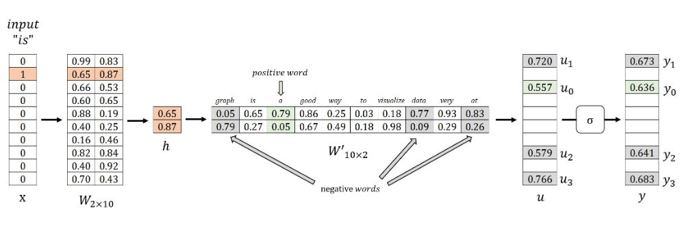
使用负采样时， $Skip$-$gram$ 模型使用 $Softmax$ 函数的以下变体，该函数实际上是 $Sigmoid$ 函数 $σ$ 的 $u_j$ 。此函数映射 $u$ :

\[y_j=\sigma(u_j)=\frac{1}{1+e^{-u_j}} \]

反向传播

如上所述，$Positive Word$ 的输出表示为 $y_0$，应为 $1$ ；虽然 $k$ 对应于负数词的输出，表示为 $y_i$，都应为 $0$ 。因此，模型训练的目标是最大化 $y_0$ 和 $1-y_i$，可以等效地解释为最大化乘积：

\[\begin{aligned}maxy_{0}&\prod_{i=1}^{k}(1-y_{i})=max\left(logy_{0}\prod_{i=1}^{k}(1-y_{i})\right)\\&=max\left(logy_{0}+\sum_{i=1}^{k}log(1-y_{i})\right)\\&=max\left(log\sigma(u_{0})+\sum_{i=1}^{k}log(1-\sigma(u_{i}))\right)\\&=max\left(log\sigma(v_{wI}\cdot{v_{w_{0}}^{^{\prime}}}^{T})+\sum_{i=1}^{k}log\sigma(-v_{wI}\cdot{v_{w_{i}}^{^{\prime}}}^{T})\right)\end{aligned} \]

损失函数 $E$ 通过将其转换为最小化问题来获得：

\[\mathrm{E}=-log\sigma\left(v_{wI}\cdot{v_{w_0}^{^{\prime}}}^T\right)-\sum_{i=1}^klog\sigma(-v_{wI}\cdot{v_{w_i}^{^{\prime}}}^T) \]

求偏导：

\[\begin{aligned}\frac{\partial E}{\partial u_{0}}&=-\frac{\partial}{\partial u_{0}}log\sigma(u_{0})=-\frac{1}{\sigma(u_{0})}\cdot\frac{\partial}{\partial u_{0}}\sigma(u_{0})\\&=-(1+e^{-u_{0}})\cdot\frac{\partial}{\partial u_{0}}\frac{1}{1+e^{-u_{0}}}\\&=-(1+e^{-u_{0}})\cdot\left(-\frac{1}{(1+e^{-u_{0}})^{2}}\right)\cdot\frac{\partial}{\partial u_{0}}e^{-u_{0}}\\&=\frac{1}{1+e^{-u_{0}}}\cdot(-e^{-u_{0}})=\frac{1}{1+e^{-u_{0}}}-1=y_{0}-1\end{aligned} \]

\[\begin{align*} \frac{\partial E}{\partial u_{i}} &= -\frac{\partial}{\partial u_{i}}\log\left(1-\sigma(u_{i})\right) \\ &= -\frac{\partial}{\partial u_{i}}\log\sigma(-u_{i}) \\ &= -\frac{1}{\sigma(-u_{i})}\cdot\frac{\partial}{\partial u_{i}}\sigma(-u_{i}) \\ &= -(1+e^{u_{i}})\cdot\frac{\partial}{\partial u_{i}}\frac{1}{1+e^{u_{i}}} \\ &= -(1+e^{u_{i}})\cdot\left(-\frac{1}{(1+e^{u_{i}})^{2}}\right)\cdot\frac{\partial}{\partial u_{i}}e^{u_{i}} \\ &= \frac{1}{1+e^{u_{i}}}\cdot e^{u_{i}} \\ &= \frac{1}{1+e^{-u_{i}}} \\ &= y_{i} \end{align*}\]

$∂E/∂u_0$ 和 $∂E/∂u_i$ 类似 $∂E/∂u_j$ 在优化前 $Skip$-$gram$ 模型中的作用，理解为从输出向量中减去期望向量：

更新矩阵中权重的过程 $W^′$ 和 $W$ 参考 $Skip$-$gram$ 的原始形式。但是，只有权重 $w_{11}^{^{\prime}},w_{21}^{^{\prime}},w_{13}^{^{\prime}},w_{23}^{^{\prime}},w_{18}^{^{\prime}},w_{28}^{^{\prime}},w_{1,10}^{^{\prime}}$ 和 $w_{2,10}^{^{\prime}}$ 在 $W^′$ 和权重 $w_{21}$ 在 $W$ 更新。

分层 $Softmax$

霍夫曼树

在分层 $softmax$ 的 $Skip$-$gram$ 中霍夫曼树是基于词频的最优二叉树，其叶子节点表示词汇表中所有单词，而在输出层中霍夫曼树的内部节点向量由神经元权重矩阵中的向量 $θ_i$ 表示。

~HuffmanFree

分层 $Softmax$ 处理

$HuffmanFree$ 将全局 $Softmax$ 分解为路径上的二分类链，通过路径查找对应上下文词的出现概率：

\[P(u|w)=\prod_{j=2}^{l^u}\begin{cases}\sigma(x_w^T\theta_{j-1}^u)&\text{向左分支}\\1-\sigma(x_w^T\theta_{j-1}^u)&\text{向右分支}&\end{cases} \]

即从根节点开始，根据 $σ(x_w^Tθ)$ 选择左/右分支，沿路径迭代，直至到达目标词 u 的叶节点。

计算效率优化对比：

`对比项`	`原始Softmax`	`霍夫曼分层Softmax`
`计算复杂度`	`O(V⋅d)`	`O(logV⋅d)`
`参数更新量`	`更新 V 个输出向量`	`更新 logV 个节点`

符号定义

$x_w$：中心词 $w$ 的输入向量（投影层输出）
$u$：目标上下文词
$l^u$：从根节点到 $u$ 的路径节点数（含根节点和叶节点）
$n(u,k)$：路径上第 $k$ 个节点（ $k=1$ 为根节点）
$θ_{k−1}^u$：节点 $n(u,k)$ 的向量表示（非叶节点）
$d_j^u∈{0,1}$：节点 $n(u,j)$ 的 $Huffman$ 编码（方向标记）

正向传播

给定中心词w和目标词u，条件概率分解为路径决策连乘：

\[P(u|w)=\prod_{j=2}^{l^u}p(d_j^u|x_w,\theta_{j-1}^u) \]

其中每个节点决策概率由Sigmoid函数定义：

\[p(d_j^u|\cdot)=\begin{cases}\sigma(x_w^T\theta_{j-1}^u)&\mathrm{if~}d_j^u=0\text{(左分支)}\\1-\sigma(x_w^T\theta_{j-1}^u)&\mathrm{if~}d_j^u=1\text{(右分支)}&\end{cases} \]

统一形式：

\[P(u|w)=\prod_{j=2}^{l^u}\left[\sigma(x_w^T\theta_{j-1}^u)\right]^{1-d_j^u}\left[1-\sigma(x_w^T\theta_{j-1}^u)\right]^{d_j^u} \]

示例（中心词="hierarchical"，目标词="model"）：

\[P(\mathrm{model}|\text{hierarchical})=(1-\sigma(x_w^T\theta_1))\cdot(1-\sigma(x_w^T\theta_2))\cdot\sigma(x_w^T\theta_3) \]

反向传播

目标函数

\[\mathrm{L}=\sum_{w\in C}\sum_{u\in\mathrm{Context}(w)}\sum_{j=2}^{l^u}\left[(1-d_j^u)\log\sigma(x_w^T\theta_{j-1}^u)+d_j^u\log(1-\sigma(x_w^T\theta_{j-1}^u))\right] \]

梯度计算

\[\theta_{j-1}^u\leftarrow\theta_{j-1}^u+\eta\begin{bmatrix}1-d_j^u-\sigma(x_w^T\theta_{j-1}^u)\end{bmatrix}x_w \]

对节点向量 $θ_{j−1}^u$ 的梯度：

\[\frac{\partial\mathrm{L}}{\partial\theta_{j-1}^u}=\begin{bmatrix}1-d_j^u-\sigma(x_w^T\theta_{j-1}^u)\end{bmatrix}x_w \]

更新规则：

\[\theta_{j-1}^u\leftarrow\theta_{j-1}^u+\eta\left[1-d_j^u-\sigma(x_w^T\theta_{j-1}^u)\right]x_w \]

对中心词向量 $x_w$ 的梯度：

\[\frac{\partial\mathrm{L}}{\partial x_w}=\sum_{j=2}^{l^u}\left[1-d_j^u-\sigma(x_w^T\theta_{j-1}^u)\right]\theta_{j-1}^u \]

更新规则：

\[x_w\leftarrow x_w+\eta\sum_{j=2}^{l^u}\left[1-d_j^u-\sigma(x_w^T\theta_{j-1}^u)\right]\theta_{j-1}^u \]

代码展示

数据处理

import numpy as np
import matplotlib.pyplot as plt
from sklearn.decomposition import PCA

corpus = '''Mechanic repairs broken engine. Farmer harvests ripe crops. Musician plays soulful melody. Mother comforts crying baby. Gardener plants colorful flowers.'''

def training_data_generator(corpus, window_size):   
    # Indexing and Vocabulary Generation
    sentences = corpus.split('.')
    indexed_sentences = []
    vocab = {}
    vocab_idx = -1
    for i in range(len(sentences)):
        sentences[i] = sentences[i].strip().split()
        if len(sentences[i]) > 0:
            indexed_sentences.append([])
            for j in range(len(sentences[i])):
                sentences[i][j] = sentences[i][j].lower()
                if sentences[i][j] not in vocab:
                    vocab_idx +=1
                    vocab[sentences[i][j]] = vocab_idx
                    indexed_sentences[-1].append(vocab_idx)
                else:
                    indexed_sentences[-1].append(vocab[sentences[i][j]])
    vocab_size = len(vocab)

    # Training Dataset Generation
    X_train = []
    y_train = []
    for i in range(len(indexed_sentences)):
        for j in range(len(indexed_sentences[i])):
            for k in range(1, window_size+1):
                center_word_ohe_vector = np.zeros(vocab_size)
                center_word_ohe_vector[indexed_sentences[i][j]] = 1
                zeros_vector = np.zeros(vocab_size)
                c_left_idx = j - k
                if c_left_idx >= 0:
                    X_train.append(center_word_ohe_vector)
                    y_train.append(np.copy(zeros_vector))
                    y_train[-1][indexed_sentences[i][c_left_idx]] = 1
                c_right_idx = j + k
                if c_right_idx < len(indexed_sentences[i]):
                    X_train.append(center_word_ohe_vector)
                    y_train.append(np.copy(zeros_vector))
                    y_train[-1][indexed_sentences[i][c_right_idx]] = 1
                    
    X_train = np.array(X_train)
    y_train = np.array(y_train)
    return X_train, y_train, vocab

X_train, y_train, vocab = training_data_generator(corpus,2)
print('First five words in vocabulary: ', list(vocab.keys())[:5])
total_training_examples, vocab_size = X_train.shape
print(f'Total training examples: {total_training_examples}')
print(f'OHE vector size / Vocabulary size: {vocab_size}')

training_data_generator函数用于处理给定的语料库corpus，通过已知的滑动窗口大小进行采样以生成模型训练要使用的单词对X_train，y_train以及语料库对应的词典vocab。

$Adam$优化

class AdamOptimizer:
    def __init__(self, alpha, params, beta1=0.9, beta2=0.999, epsilon=10e-8):
        self.alpha = alpha
        self.beta1 = beta1
        self.beta2 = beta2
        self.epsilon = epsilon
        self.moments = []
        self.epoch = 0
        if not params:
            raise Exception("Parameters can't be undefined!")
        for i in range(len(params)):
            self.moments.append(
                {
                    'V': np.zeros_like(params[i]),
                    'S': np.zeros_like(params[i])
                }
            )

    def update(self, params=[], grads=[]):
        params_len = len(params)
        grads_len = len(grads)
        if params_len != grads_len or params_len == 0:
            raise Exception("Empty or Inconsistant Parameters and Gradients List!")

        self.epoch += 1

        for i in range(grads_len):
            # Update biased first moment estimate
            self.moments[i]['V'] = self.beta1 * self.moments[i]['V'] + (1 - self.beta1) * grads[i]
            # Update biased second raw moment estimate (RMSProp part)
            self.moments[i]['S'] = self.beta2 * self.moments[i]['S'] + (1 - self.beta2) * np.square(grads[i])
            # Compute bias-corrected first moment estimate
            VdW_corrected = self.moments[i]['V'] / (1 - self.beta1 ** self.epoch)
            # Compute bias-corrected second raw moment estimate (RMSProp part)
            SdW_corrected = self.moments[i]['S'] / (1 - self.beta2 ** self.epoch)
            # Update parameters
            params[i] -= self.alpha * VdW_corrected / (np.sqrt(SdW_corrected) + self.epsilon)
        
        return params

这里类AdamOptimizer实现了 Adam（Adaptive Moment Estimation）优化算法，这是一种广泛用于深度学习的自适应学习率优化器。它结合了动量梯度下降（Momentum）和 RMSProp 的优点，通过自适应调整每个参数的学习率来加速模型收敛。

初始化方法 __init__:

参数：
- alpha：基础学习率 (步长)
- params：需要优化的模型参数（权重矩阵/偏置向量等）
- beta1/beta2：指数衰减率（默认值分别为0.9和0.999）
- epsilon：数值稳定常数（防止除零）
初始化：
- 为每个参数创建动量累积器（V：一阶矩/动量）
- 为每个参数创建RMS累积器（S：二阶矩/未中心化的方差）
- 训练轮次计数器 epoch

更新方法 update:

输入：当前参数值 params 和对应梯度 grads
执行关键操作：

循环遍历每个参数：

V = β1·V + (1-β1)·grad      ← 动量更新（类似带摩擦的物理运动）
S = β2·S + (1-β2)·grad²      ← 自适应学习率更新（梯度平方）
V̂ = V / (1-β1^epoch)        ← 偏差校正（补偿初始0值）
Ŝ = S / (1-β2^epoch)        ← 偏差校正

param = param - α·V̂/(√Ŝ + ε) ← 参数更新

返回更新后的参数列表

$SkipGram$

class SkipGram:
    def __init__(self, embedding_size, vocab):
        self.vocab = vocab
        self.vocab_rev = {v: k for k, v in vocab.items()}   # Used in finding context words using cosine similarity
        self.vocab_size = len(vocab)
        self.embedding_size = embedding_size
        self.reset_weights()

    def softmax(self, H):
        Yhat = np.exp(H - np.max(H, axis=0))    # Subtracting max logit to avoid overflow and underflow
        return Yhat / Yhat.sum(axis=0)

    def reset_weights(self):
        self.W = np.random.randn(self.vocab_size, self.embedding_size) * np.sqrt(2 / (self.vocab_size + self.embedding_size))
        self.Wprime = np.random.randn(self.embedding_size, self.vocab_size) * np.sqrt(2 / (self.embedding_size + self.vocab_size))
        return

    def update(self, total_training_examples, dL_by_dW, dL_by_dWprime):
        norm = 1/total_training_examples

        dL_by_dW *= norm
        dL_by_dWprime *= norm

        self.W, self.Wprime = self.optimizer.update(params=[self.W, self.Wprime], grads=[dL_by_dW, dL_by_dWprime])

        return
    
    def forward_prop(self, X_train):
        H = self.W.T @ X_train
        U = self.Wprime.T @ H
        Yhat = self.softmax(U)
        return H, Yhat
    
    def backprop(self, X_train, Y_train, H, Yhat):
        temp = Yhat - Y_train
        dL_by_dWprime = H @ temp.T
        dL_by_dW = X_train @ (self.Wprime @ temp).T
        return dL_by_dW, dL_by_dWprime

    def calc_cce(self, Yhat, true_labels):
        # Clip y_pred to avoid log(0) and very small values that may cause numerical instability
        Yhat = np.clip(Yhat, 1e-15, 1 - 1e-15)

        total_loss = -np.sum(true_labels * np.log(Yhat+10e-10))

        return total_loss
    
    def cosine_similarity(self, v1, v2):
        """
        Parameters:
        - v1, v2: NumPy arrays representing the word embeddings of two words.
        
        Returns:
        - cosine_similarity: A scalar value representing the cosine similarity between the two vectors.
        """
        dot_product = np.dot(v1, v2)
        norm_v1 = np.linalg.norm(v1)
        norm_v2 = np.linalg.norm(v2)
        return dot_product / (norm_v1 * norm_v2)
    
    def get_context_words(self, word, num_context_words):
        word = word.lower()
        if word not in vocab:
            raise ValueError(f"Word '{word}' not found in the vocabulary.")

        # Get the index of the center word
        center_word_idx = vocab[word]
        
        # Get the embedding of the center word
        center_embedding = self.W[center_word_idx]

        # Compute cosine similarity between the center word and all other words
        similarities = []
        for idx, context_embedding in enumerate(self.W):
            if idx != center_word_idx:  # Skip the center word
                similarity = self.cosine_similarity(center_embedding, context_embedding)
                similarities.append((idx, similarity))

        # Sort the context words based on similarity in descending order
        similarities.sort(key=lambda x: x[1], reverse=True)

        # Return the top 'num_context_words' context words
        context_words_with_sim = [(self.vocab_rev[idx], similarity) for idx, similarity in similarities[:num_context_words]]
        return context_words_with_sim

    def train(self, X_train, Y_train, epochs, lr=0.1):
        X_train = X_train.T
        Y_train = Y_train.T
        total_training_examples = X_train.shape[-1]
        training_loss_history = []
        self.reset_weights()
        self.optimizer = AdamOptimizer(alpha=lr, params=[self.W, self.Wprime])
        for epoch in range(epochs):
            dL_by_dW = np.zeros((self.vocab_size, self.embedding_size))
            dL_by_dWprime = np.zeros((self.embedding_size, self.vocab_size))
            H, Yhat = self.forward_prop(X_train)
            dL_by_dW, dL_by_dWprime = self.backprop(X_train, Y_train, H, Yhat)
            self.update(total_training_examples, dL_by_dW, dL_by_dWprime)
            loss = self.calc_cce(Yhat, Y_train) / total_training_examples
            training_loss_history.append(loss)
            print(f"Epoch {epoch+1:03d} | " f"Training Loss (CCE): {loss:.4f}")
        return training_loss_history

sg = SkipGram(embedding_size=5, vocab=vocab)

SkipGram 类完整实现了 $Skip$-$gram$ 词向量模型，学习单词的分布式表示。
1. __init__(self, embedding_size, vocab)

功能: 模型初始化

存储词汇表和创建反向映射
记录词汇大小和嵌入维度
调用 reset_weights() 初始化权重矩阵

self.vocab = vocab
self.vocab_rev = {v: k for k, v in vocab.items()}  # 索引→单词的映射
self.vocab_size = len(vocab)
self.embedding_size = embedding_size
self.reset_weights()  # 初始化权重矩阵

2. softmax(self, H)

功能: 数值稳定的 softmax 计算

减去最大值避免指数溢出
指数化并归一化概率分布

Yhat = np.exp(H - np.max(H, axis=0))  # 数值稳定处理
return Yhat / Yhat.sum(axis=0)  # 概率归一化

3. reset_weights(self)

功能: 权重初始化 (Xavier/Glorot 初始化)

使用正态分布初始化权重
根据输入/输出维度调整初始方差

scale = np.sqrt(2 / (self.vocab_size + self.embedding_size))
self.W = np.random.randn(self.vocab_size, self.embedding_size) * scale
self.Wprime = np.random.randn(self.embedding_size, self.vocab_size) * scale

4. update(self, total_training_examples, dL_by_dW, dL_by_dWprime)

功能: 参数更新

梯度归一化（除以样本量）
调用 Adam 优化器更新权重

norm = 1 / total_training_examples  # 梯度平均因子
dL_by_dW *= norm
dL_by_dWprime *= norm
# 调用优化器更新权重
self.W, self.Wprime = self.optimizer.update(params=[self.W, self.Wprime], 
                                           grads=[dL_by_dW, dL_by_dWprime])

5. forward_prop(self, X_train)

功能: 前向传播计算

词嵌入计算
上下文预测输出
Softmax 概率分布

H = self.W.T @ X_train        # 输入→隐藏：词向量生成
U = self.Wprime.T @ H         # 隐藏→输出：上下文预测
Yhat = self.softmax(U)        # 概率分布
return H, Yhat

6. backprop(self, X_train, Y_train, H, Yhat)

功能: 反向传播计算梯度

计算输出层误差
计算隐藏层到输出层梯度
计算输入层到隐藏层梯度

temp = Yhat - Y_train  # 输出层误差
dL_by_dWprime = H @ temp.T  # W' 梯度：隐藏→输出层
dL_by_dW = X_train @ (self.Wprime @ temp).T  # W 梯度：输入→隐藏层
return dL_by_dW, dL_by_dWprime

7. calc_cce(self, Yhat, true_labels)

功能: 分类交叉熵损失计算

概率裁剪防止数值溢出
交叉熵损失计算

Yhat = np.clip(Yhat, 1e-15, 1 - 1e-15)  # 数值稳定处理
total_loss = -np.sum(true_labels * np.log(Yhat))  # 交叉熵计算
return total_loss

8. cosine_similarity(self, v1, v2)

功能: 余弦相似度计算

点积计算
向量规范化
相似度计算

dot_product = np.dot(v1, v2)
norm_v1 = np.linalg.norm(v1)
norm_v2 = np.linalg.norm(v2)
return dot_product / (norm_v1 * norm_v2)  # 余弦相似度

9. get_context_words(self, word, num_context_words)

功能: 寻找相似上下文词

获取中心词索引和词向量
计算与所有词的相似度
排序并返回最相似的词

center_word_idx = vocab[word.lower()]  # 获取索引
center_embedding = self.W[center_word_idx]  # 获取词向量

# 计算所有相似度
similarities = []
for idx, embedding in enumerate(self.W):
    if idx != center_word_idx:
        similarity = self.cosine_similarity(center_embedding, embedding)
        similarities.append((idx, similarity))

# 返回最相似的上下文词
return [(self.vocab_rev[idx], sim) for idx, sim in 
        sorted(similarities, key=lambda x: x[1], reverse=True)[:num_context_words]]

10. train(self, X_train, Y_train, epochs, lr=0.1)

功能: 模型训练主循环

数据预处理
优化器初始化
迭代训练：
- 前向传播
- 反向传播
- 参数更新
- 损失计算

X_train = X_train.T; Y_train = Y_train.T  # 维度转置
total_examples = X_train.shape[-1]
self.reset_weights()
self.optimizer = AdamOptimizer(alpha=lr, params=[self.W, self.Wprime])

for epoch in range(epochs):
    # 梯度清零
    dL_by_dW = np.zeros_like(self.W)
    dL_by_dWprime = np.zeros_like(self.Wprime)
    
    # 前向传播
    H, Yhat = self.forward_prop(X_train)
    
    # 反向传播
    dL_by_dW, dL_by_dWprime = self.backprop(X_train, Y_train, H, Yhat)
    
    # 参数更新
    self.update(total_examples, dL_by_dW, dL_by_dWprime)
    
    # 损失计算和记录
    loss = self.calc_cce(Yhat, Y_train) / total_examples
    training_loss_history.append(loss)

$PCA$可视化处理

# For visualization of word embeddings before training

# Apply PCA to reduce to 2 dimensions
pca = PCA(n_components=2)
data_2d = pca.fit_transform(sg.W)

# Reverse the dictionary to map indices to words for labeling in the plot
index_to_word = {index: word for word, index in vocab.items()}

# Plot the data with words as labels
plt.figure(figsize=(11, 7.3))

color_list = ['blue', 'blue', 'blue', 'blue', 'green', 'green', 'green', 'green', 'red', 'red', 'red', 'red', 'orange', 'orange', 'orange', 'orange', 'magenta', 'magenta', 'magenta', 'magenta']

for idx, (x, y) in enumerate(data_2d):
    plt.scatter(x, y, color=color_list[idx], alpha=1.0, edgecolor='k')

# Now, use the adjusted label positions
for idx, (x, y) in enumerate(data_2d):
    plt.text(x + 0.02, y + 0.02, index_to_word[idx], color=color_list[idx], fontsize=14)

plt.grid()
plt.title("2D Visualization of Word Embeddings Before Training", fontsize=25)
plt.xlabel("Principal Component 1", fontsize=20)
plt.ylabel("Principal Component 2", fontsize=20)
# plt.savefig("word embedding before training.png", dpi=300)
plt.tight_layout()
plt.show()
plt.save()

PCA降维处理：

pca = PCA(n_components=2)
data_2d = pca.fit_transform(sg.W)

使用PCA（主成分分析）将高维词向量（sg.W）降至2D，便于可视化
fit_transform()同时完成模型拟合和数据转换

索引到单词映射：

index_to_word = {index: word for word, index in vocab.items()}

创建反向词汇表（索引→单词的映射），用于在图上标注单词
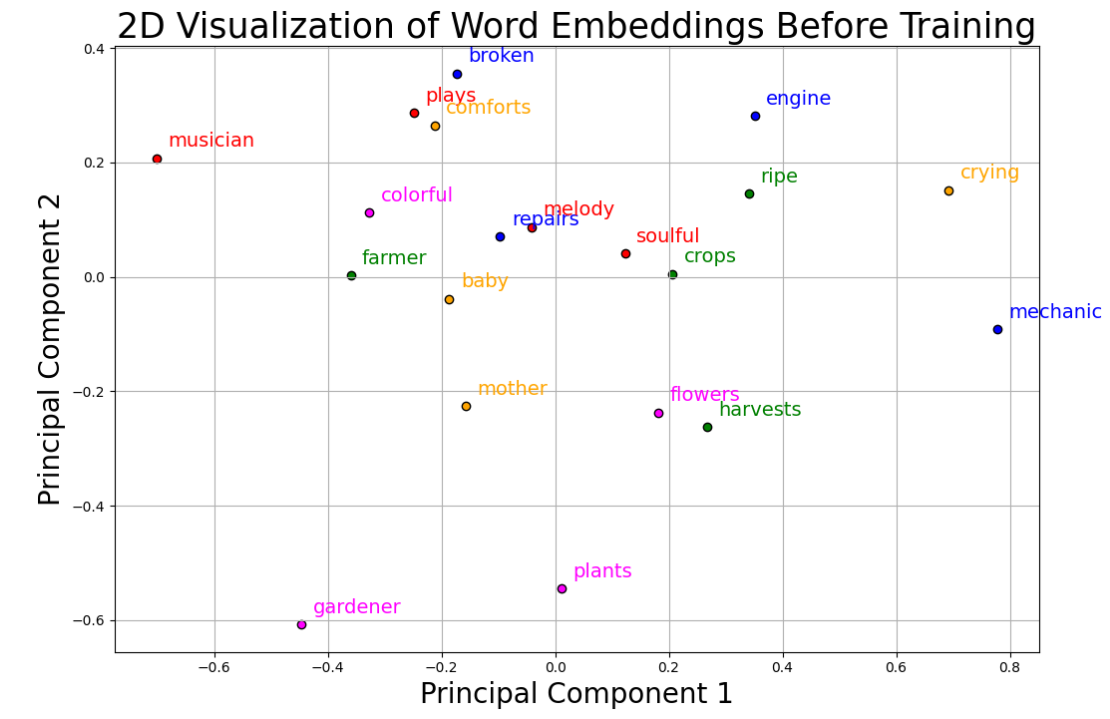
对原始初始化词向量结果进行PCA的降维结果如下所示：

~beforePCA

模型训练过程中的损失函数变化：

training_loss_history = sg.train(X_train, y_train, 50, lr=0.1)

iterations = np.arange(1, len(training_loss_history)+1)
plt.figure(figsize=(9, 6))
plt.plot(iterations, training_loss_history, linewidth=2)
plt.title('Categorical Cross Entropy vs Epochs', fontsize=25)
plt.xlabel('Epoch', fontsize=20)
plt.ylabel('Categorical Cross Entropy', fontsize=20)
plt.xticks(fontsize=16)
plt.yticks(fontsize=16)
plt.grid(True)
plt.tight_layout()
# plt.savefig('cce_skipgram.png', dpi=300)
plt.show()
plt.save()

~lossF

# For visualization of word embeddings after training

# Apply PCA to reduce to 2 dimensions
pca = PCA(n_components=2)
data_2d = pca.fit_transform(sg.W)  # Assuming sg.W is your word embeddings

# Reverse the dictionary to map indices to words for labeling in the plot
index_to_word = {index: word for word, index in vocab.items()}

# Define a minimum distance to maintain between labels
min_distance = 0.7

# Create a list to store the final adjusted text label positions
adjusted_text_positions = np.copy(data_2d)

# Function to adjust text label positions if they are too close
def adjust_text_positions(positions, min_distance):
    adjusted_positions = np.copy(positions)
    for i in range(len(positions)):
        for j in range(i + 1, len(positions)):
            # Calculate the Euclidean distance between the text label positions
            dist = np.linalg.norm(adjusted_positions[i] - adjusted_positions[j])
            
            # If the distance is too small, adjust the positions of the labels
            if dist < min_distance:
                # Calculate the direction vector
                direction = adjusted_positions[i] - adjusted_positions[j]
                # Normalize the direction vector
                direction /= np.linalg.norm(direction)
                
                # Move the labels apart by the necessary amount (displacement)
                displacement = (min_distance - dist) / 2
                adjusted_positions[i] += direction * displacement
                adjusted_positions[j] -= direction * displacement
    return adjusted_positions

# Adjust the text label positions to ensure they do not overlap
adjusted_text_positions = adjust_text_positions(adjusted_text_positions, min_distance)

# Plot the data with words as labels
plt.figure(figsize=(11, 7.3))

color_list = ['blue', 'blue', 'blue', 'blue', 'green', 'green', 'green', 'green', 'red', 'red', 'red', 'red', 'orange', 'orange', 'orange', 'orange', 'magenta', 'magenta', 'magenta', 'magenta']

for idx, (x, y) in enumerate(data_2d):
    plt.scatter(x, y, color=color_list[idx], alpha=1.0, edgecolor='k')

# Now, use the adjusted label positions
for idx, (x, y) in enumerate(adjusted_text_positions):
    plt.text(x + 0.02, y + 0.02, index_to_word[idx], color=color_list[idx], fontsize=15)

plt.grid()
plt.title("2D Visualization of Word Embeddings After Training", fontsize=25)
plt.xlabel("Principal Component 1", fontsize=20)
plt.ylabel("Principal Component 2", fontsize=20)
# plt.savefig("word embedding after training.png", dpi=300)
plt.tight_layout()
plt.show()
plt.save()

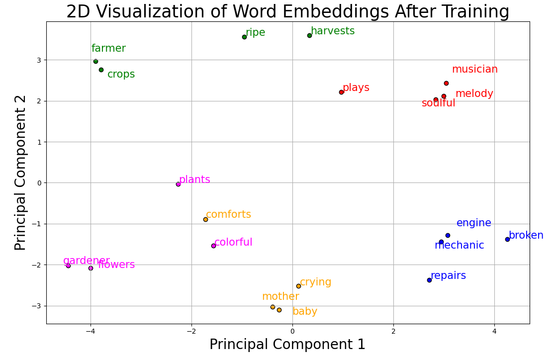
对训练后的模型对应的此嵌入向量进行PCA降维的结果：

~afterPCA

对当前嵌入向量的结果进行测试：

center_word = "mother"
context_words = sg.get_context_words(center_word, num_context_words=3)
print(f"Context words for target word '{center_word}' are:")
print(context_words)

Context words for target word 'mother' are:
[('baby', 0.9924191032897455), ('plants', 0.4663178819947096), ('flowers', 0.37168944028566714)]

参考

posted @ 2025-07-08 17:38 StuBoo 阅读(138) 评论(0) 收藏举报

刷新页面返回顶部

stuBoo

Node2Vec、Word2Vec中Skip Gram的超详细解析

概述

\(Skip\) \(Gram\) 模型

模型概述

余弦相似度

语料库 \(Corpus\)

滑动窗口采样

\(One\)-\(hot\) 编码

\(Skip\)-\(gram\) 架构

前向传播

\(Input Layer → Hidden Layer\)

\(Hidden Layer → Output Layer\)

反向传播

权重更新机制

损失函数定义

\(Output Layer → Hidden Layer\)

\(Hidden Layer → Input Layer\)

\(Skip\)-\(gram\) 优化

子采样

负采样

优化后的模型训练

前向传播

反向传播

分层 \(Softmax\)

霍夫曼树

分层 \(Softmax\) 处理

符号定义

正向传播

反向传播

代码展示

数据处理

\(Adam\)优化

\(SkipGram\)

\(PCA\)可视化处理

参考

公告

stuBoo

Node2Vec、Word2Vec中Skip Gram的超详细解析

概述

\(Skip\) \(Gram\) 模型

模型概述

余弦相似度

语料库 \(Corpus\)

滑动窗口采样

\(One\)-\(hot\) 编码

\(Skip\)-\(gram\) 架构

前向传播

\(Input Layer → Hidden Layer\)

\(Hidden Layer → Output Layer\)​

反向传播

权重更新机制

损失函数定义

\(Output Layer → Hidden Layer\)

\(Hidden Layer → Input Layer\)

\(Skip\)-\(gram\) 优化

子采样

负采样

优化后的模型训练

前向传播

反向传播

分层 \(Softmax\)

霍夫曼树

分层 \(Softmax\) 处理​

符号定义

正向传播

反向传播

代码展示

数据处理

\(Adam\)优化

\(SkipGram\)

\(PCA\)可视化处理

参考

公告

\(Hidden Layer → Output Layer\)

分层 \(Softmax\) 处理