

Time Series_4_Volatility
1. Cointegrated VAR and Vector Error Correction Model (VECM)
1.1 传统VAR要求variables是stationary,实际上不同股票会被同样基本面驱动。若按常规,在cointegrated series的背景下use first differentiate to remove unit root model会导致overdifferencing并丧失许多信息,尤其是long-term comovement of variable levels。故而使用VECM:consists of VAR model of (1) the order (p-1) on the differences of variables, and (2) an error-correction term derived from the known(estimated) cointegrating relationship。
e.g., in stock market, VECM establishes short-term relationship between stock returns, while correcting with deviation from long-term comovement of prices.
1.2 Two variable: Engle-Granger;
Multivariate: Johansen procedure
1.3 Case
library(quantmod)
getSymbols('DTB3', src = 'FRED')
getSymbols('DTB6', src = 'FRED')
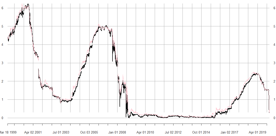
DTB3.sub = DTB3['1999-03-18/2020-03-18']
DTB6.sub = DTB6['1999-03-18/2020-03-18']
plot(DTB3.sub)
lines(DTB6.sub, col = 'pink')
1.3.1 Mistake to Use Traditional ADF
Run linear regression to estimate cointegratign relationship. If residuals is stationary series, then the two series are cointegrated.
a = as.numeric(na.omit(DTB3.sub))
b = as.numeric(na.omit(DTB6.sub))
y = cbind(a, b)
cointregr <- lm(a ~ b)
r = cointregr$residuals
library(urca)
summary(ur.df(r,type = 'none'))
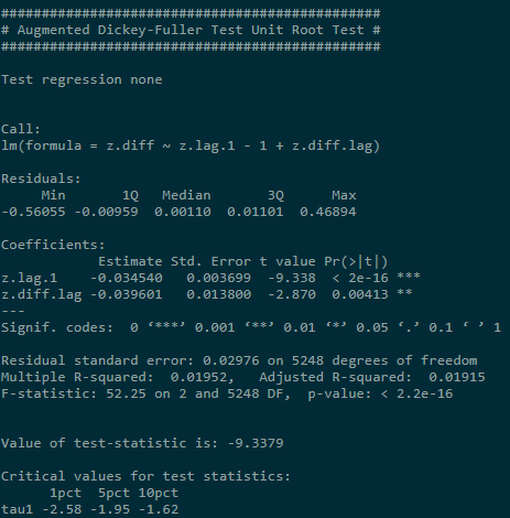
ADF tests indicate that NULL of unit root cannot be rejected. But in our case, conventional critical values are not appropriate, 需要修正变量。
1.3.2 Phillips and Ouliaris test (考虑了cointegration)
NULL: Two series are not cointegrated.
Result shows low p-value, indicating rejection of NULL, i.e. there exisit cointegration.
library(tseries)
pocointregr <- po.test(y, demean = T, lshort = T)
pocointregr$parameter

1.3.3 Johansen Procedure test
# K is lag order
johansentest <- ca.jo(y, type = c('trace'), ecdet = c('none'), K = 2)
summary(johansentest)
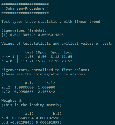
The test statistic for r = 0 is 113.71 > critical, indicating rejection of NULL; for r ≤ 1, cannot reject NULL. Thus, conclude that one cointegrating relationship exists.
1.3.4 Obtain VECM representation (run OLS on lagged differenced variables and the error correction term derived from previously calculated cointegrating relationship)
yJoregr = cajorls(johansentest, r = 1)
yJoregr

The coefficient of error-correction term is negative: short-term deviation from long-term equilibrium level would push variables to zero-equilibrium deviation.
2. Volatility Modeling
(1) Volatility Clustering;
(2) Non-normality of Asset Returns (fat tails);
(3) Leverage Effect (σ reacts differently to positive or negative price movements, 价格下降带来的σ 变动幅度更大);
2.1 Case S&P
getSymbols('SNP',from = '2008-03-18', to = Sys.Date(), env = data_env)
data_env <- new.env()
snp <- do.call(merge, eapply(data_env, Cl))
head(snp)
library(fImport)
ret <- dailyReturn(snp$SNP.Close, type = 'log')
par(mfrow = c(2, 2))
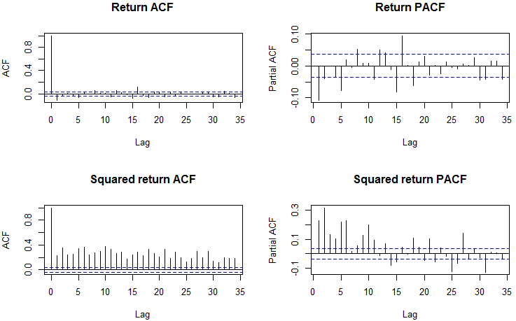
acf(ret, main = 'Return ACF');
pacf(ret, main = 'Return PACF');
acf(ret^2, main = 'Squared return ACF');
pacf(ret^2, main = 'Squaredreturn PACF');
par(mfrow = c(1, 1))
We expect log returns to be serially uncorrelated, while results below the squared or absolute log returns show significant autocorrelations, which means that log returns are not correlated,but not independent.
m = mean(ret)
s = sd(ret)
par(mfrow = c(1,2))
hist(ret, nclass = 40, freq = F, main = 'Return histograms')
curve(dnorm(x, mean = m, sd = s), from = -0.3,
      to = 0.2, add = T, col = 'brown')
plot(density(ret), main = 'Return empirical distribution')
curve(dnorm(x, mean = m, sd = s), from = -0.3,
      to = 0.2, add = T, col = 'brown')
par(mfrow = c(1, 1))

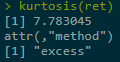
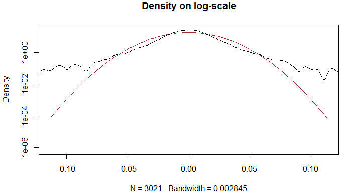
Fat tail and excess kurtosis exisit.
kurtosis(ret)
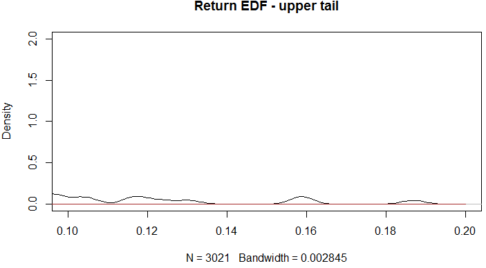
# Zoom in fat tail
plot(density(ret), main = 'Return EDF - upper tail',
     xlim = c(0.1, 0.2), ylim = c(0, 2))
curve(dnorm(x, m, s),from = -0.3,
      to = 0.2, add = T, col = 'brown')
# density on log-scale
plot(density(ret), xlim = c(-5*s, 5*s), log = 'y',
     main = 'Density on log-scale')
curve(dnorm(x, m, s), from = -5*s, to = 5*s, log = 'y',
      add = T, col = 'brown')
#qqplot depicts empirical quantiles against normal/theoretical distribution
#deviations from straight line means presence of fat tails
qqnorm(ret)
qqline(ret)

3. Modelling Volatility
3.1 Stochastic Volatility(SV)
Volatility is not measurable with respect to available information set, hence it must be filtered out from measurement equation, i.e. its own stochastic process.
3.2 GARCH-family
3.2.1 Bg Knowledge
Conditional σ2 given past observations is known.
GARCH(1,1)对称,所以不适用leverage effects or capture asymmetries distributions.
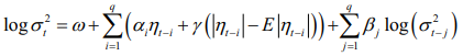
GARCH(p,q):
![]()
3.2.2 Case BRKA: GARCH(1,1)
library(rugarch)
library(quantmod)
data_env <- new.env()
getSymbols(Symbols = 'BRK-A', env = data_env,
           from = '2008-03-18', to = '2020-03-18')
close.brka <- do.call(merge, eapply(data_env, Cl))
ret.brka <- dailyReturn(close.brka, type = 'log')
plot(ret.brka)

# create a univariate object, GARCH(1,1) only one const mu
garch11.spec = ugarchspec(variance.model = list(model = 'sGARCH',
                                               garchOrder = c(1,1),
                                               mean.model = list(armaOrder = c(0,0))))
brka.garch11.fit = ugarchfit(spec = garch11.spec, data = ret.brka)
coef(brka.garch11.fit)

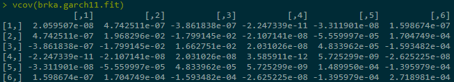
vcov(brka.garch11.fit) # covariance matrix for parameter estimates
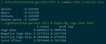
infocriteria(brka.garch11.fit) # common info criteria list
signbias(brka.garch11.fit) # Engle-Ng sign bias test
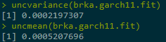
uncvariance(brka.garch11.fit) # unconditional long-term var
uncmean(brka.garch11.fit) #unconditional long-term mean
# Use News inpact curve to visualize magnitude of
# volatility changes in response to shocks
nic.garch11 <- newsimpact(brka.garch11.fit)
plot(nic.garch11$zx, nic.garch11$zy, type = 'l', lwd = 2, col = 'brown',
     main = 'GARCH(1,1) - News Impact Curve', ylab = nic.garch11$yexpr,
     xlab = nic.garch11$xexpr)
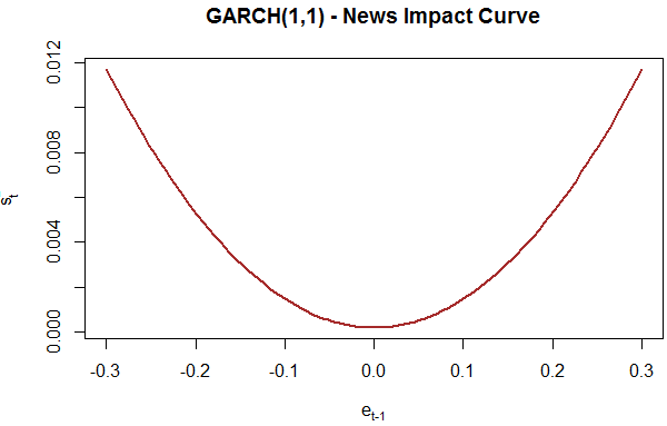
As is shown above, no asymmetries are present in response to +/- shocks.
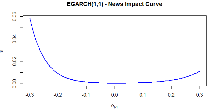
3.2.3 EGARCH
This approach models logarithm of conditional volatility, allowing multiplicative dynamics in evolving the volatility process. Asymmetry is captured by αi and negative indicates that process reacts more to negative shocks.
egarch11.spec = ugarchspec(variance.model = list(model = 'eGARCH',
                                                 garchOrder = c(1,1)),
                           mean.model = list(armaOrder = c(0,0)))
brka.egarch11.fit = ugarchfit(spec = egarch11.spec,
                              data = ret.brka)
coef(brka.egarch11.fit)

Above shows asymmetry in response of conditional volatility. Hence, asymmetric models are necessary.
nic.egarch11 <- newsimpact(brka.egarch11.fit)
plot(nic.egarch11$zx, nic.egarch11$zy, type = 'l', lwd = 2, col = 'blue',
     main = 'EGARCH(1,1) - News Impact Curve', ylab = nic.egarch11$yexpr,
     xlab = nic.egarch11$xexpr)
3.2.4 TGARCH (threshold model)
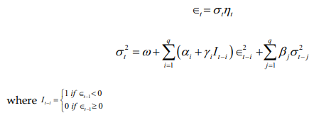
γi if positive, negative ε gonna have higher impact on conditional volatility, e.g., leverage effect.
tgarch11.spec = ugarchspec(variance.model = list(model = 'fGARCH',
                                                 submodel = 'TGARCH',
                                                 garchOrder = c(1,1)),
                           mean.model = list(armaOrder = c(0,0)))
brka.tgarch11.fit = ugarchfit(spec = tgarch11.spec, data = ret.brka)
coef(brka.tgarch11.fit)
nic.tgarch11 <- newsimpact(brka.tgarch11.fit)
plot(nic.tgarch11$zx, nic.tgarch11$zy, type = 'l', lwd = 2, col = 'green',
     main = 'TGARCH(1,1) - News Impact Curve', ylab = nic.tgarch11$yexpr,
     xlab = nic.tgarch11$xexpr)

There's a kink above.
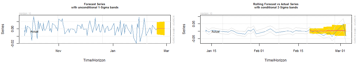
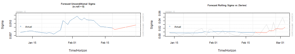
4. Simulation and Forecasting
brka.garch11.fit = ugarchfit(spec = garch11.spec,
                             data = ret.brka,
                             out.sample = 20)
brka.garch11.fcst = ugarchforecast(brka.garch11.fit, n.ahead = 10,
                                   n.roll = 10)
plot(brka.garch11.fcst, which = 'all')

 浙公网安备 33010602011771号