Time Series_1_BRKA Case

Berkshire Hathaway (The most expensive stock ever in the world)

1.1 Download data

require(quantmod)
data_env <- new.env()
getSymbols(Symbols = 'BRK-A',env = data_env)
brka_close <- do.call(merge, eapply(data_env, Cl))

 

 

1.2 Overview

1.2.1 Returns

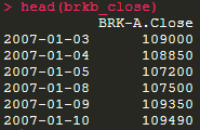
Method 1

library(fImport)
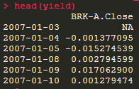
yield <- returns(brka_close)
head(yield)

Method 2

library(zoo)
# unit in percentage terms
yield_simple <- diff(brka_close) / lag(brka_close, k = -1) * 100
# coredate method: indicate we only care about price column, not the date
summary(coredata(yield_simple))

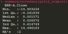
  The biggest single-day loss is 14.90%, we can find out the date by:

yield_simple[which.min(yield_simple)]

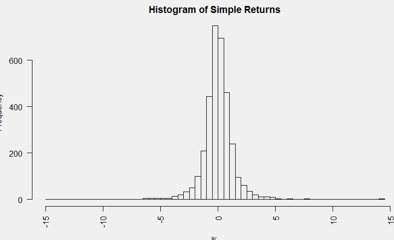
 1.2.2 Distribution of returns

hist(yield_simple, breaks = 100,
     main = 'Histogram of Simple Returns', xlab = '%')

 

1.2.3 Simple VaR calculation

 To determine the 1-day 99% VaR:

quantile(yield_simple,na.rm = T, probs = 0.01)

Thus, the prob. that yield below 3.6894% on any given day is only 1%. If that day comes, 3.6894% is the minimum amount we will lose.

1.3 Modeling the price

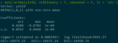
require(forecast)
mod <- auto.arima(yield, stationary = T, seasonal = F, ic = 'aic')

 

  AR(2) process didn't appear in the result below, which indicates that historic returns don't depend on earlier periods, i.e.,it depends on stochastic terms.

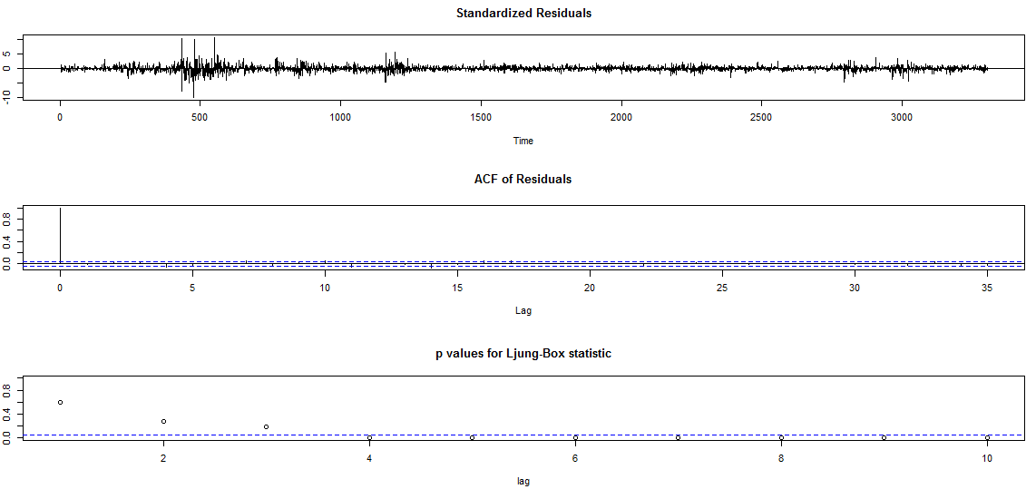
#compute confidence interval
tsdiag(mod)

Time series diagnosis below, firstly there were volatility clusters in standard residuals throughout time, secondly no autocorrelations exisit within residuals in ACF test, thirdly, Ljung-Box show p-values small to reject null hypothesis.