数据库中的window算子优化方案

window算子的基本功能理解起来较为简单，这里不再赘述，下文仅对window算子的优化方案进行说明，以下优化思路来源于http://www.vldb.org/pvldb/vol8/p1058-leis.pdf论文

对于初始的partition分区和order by排序阶段，有两种传统方法：

1、The hash-based approach fully partitions the input using hash values of the partition by attributes before sorting each partition independently using only the order by attributes.

基于Hash的方法，在使用orderby对每个分区进行独立排序之前，对partition by列进行hash分区。

2、The sort-based approach first sorts the input by both the partition by and the order by attributes. The partition boundaries are determined “on-the-fly” during the window function evaluation phase (phase 3), e.g., using binary search.

基于排序的方法，先按partition by列和order by列进行多列排序，在窗口函数求值阶段动态确定分区的边界，比如通过折半查找。

From a purely theoretical point of view, the hash-based approach is preferable. Assuming there are n input rows and O(n) partitions, the overall complexity of the hash-based approach is O(n),whereas the sort-based approach results in O(n log n) complexity.Nevertheless, the sort-based approach is often used in commercial systems—perhaps because it requires less implementation effort, as a sorting phase is always required anyway. In order to achieve good performance and scalability we use combination of both methods.

从纯理论的角度来看，基于Hash的方法更好一些。假设有n个输入行和n个分区，基于Hash方法的总体复杂度是O(n)，而基于排序方法的总体复杂度是O(n log n)。然而，商业系统中常用基于排序的方法——可能是因为实现起来比较简单，因为无论如何都需要排序阶段。为了实现更好的性能和扩展性，我们将这两种方法进行合并。

In single-threaded execution, it is usually best to first fully partition the input data using a hash table. With parallel execution, a concurrent hash table would be required for this approach. We have found, however, that concurrent, dynamically-growing hash tables (e.g., split-ordered lists [23]) have a significant overhead in comparison with unsynchronized hash tables. The sort-based approach, without partitioning first, is also very expensive. Therefore, to achieve high scalability and low overhead, we use a hybrid approach that combines the two methods。

在单线程执行时，最好首先使用Hash表对输入数据进行分区。对于并行执行，这种方法需要一个并发Hash表。然而，我们发现，与不同步的Hash表相比，并发的、动态增长的Hash表（例如，拆分有序列表）有很大的开销。基于排序的方法（不需要首先分区）也非常昂贵。因此，为了实现高可扩展性和低开销，我们使用了一种将这两种方法结合起来的混合方法。

Pre-Partitioning into Hash Groups

预先划分为Hash组

Our approach is to partition the input data into a constant number (e.g., 1024) of hash groups, regardless of how many partitions the input data has. The number of hash groups should be a power of 2 and larger than the number of threads but small enough to make partitioning efficient on modern CPUs. This form of partitioning can be done very efficiently in parallel due to limited synchronization requirements: As illustrated in Figure 3, each thread (distinguished using different colors) initially has its own array of hash groups (4 in the figure)2. After all threads have partitioned their input data, the corresponding hash groups from all threads are copied into a combined array. This can be done in parallel and without synchronization because at this point the sizes and offsets of all threads’ hash groups are known. After copying, each combined hash group is stored in a contiguous array, which allows for efficient random access to each tuple.

 

 

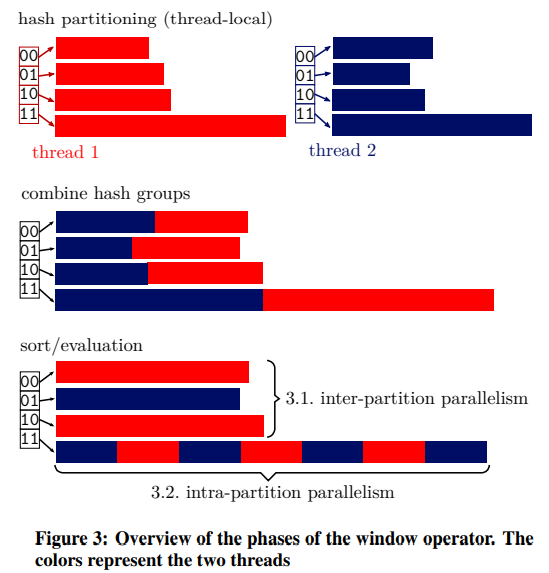
我们的方法是将输入数据划分为一个固定数目（例如1024个）的Hash组，而不管输入数据有多少个分区。Hash组的数量应该是2的幂次方，并且大于线程的数量，但要小到足以在现代cpu上有效地进行分区。由于有限的同步要求，这种形式的分区可以非常高效地并行进行：如图3所示，每个线程（使用不同的颜色区分）最初都有自己的Hash组数组（图中的4个）2。在所有线程对其输入数据进行分区之后，所有线程中相应的Hash组被复制到一个组合数组中。这可以并行进行，而不需要同步，因为此时所有线程的Hash组的大小和偏移量都是已知的。在复制之后，每个组合的Hash组都存储在一个连续的数组中，这样可以有效地随机访问每个元组。

After the hash groups copied, the next step is to sort them by both the partitioning and the ordering expressions. As a result, all tuples with the same partitioning key are adjacent in the same hash group,although of course a hash group may contain multiple partitioning keys. When necessary, the actual partition boundaries can be determined using binary search as in the sort-based approach during execution of the remaining window function evaluation step.

在复制Hash组之后，下一步是按partition by列和order by列对它们进行多列排序。因此，partition by列值相同的所有元组都在同一个Hash组中相邻，尽管当然一个Hash组可能包含多个分区键。必要时，在执行剩余的窗口函数求值步骤期间，可以使用基于排序方法中的折半查找来确定实际的分区边界。

Inter- and Intra-Partition Parallelism

分区间和分区内的并行

At first glance, the window operator seems to be embarrassingly parallel, as partitioning can be done in parallel and all hash groups are independent from each other: Since sorting and window function evaluation for different hash groups is independent, the available threads can simply work on different hash groups without needing any synchronization. Database systems that parallelize window functions usually use this strategy, as it is easy to implement and can offer very good performance for “good-natured” queries.

乍一看，window操作符似乎是令人尴尬的并行，因为分区可以并行进行，而且所有Hash组都是相互独立的：由于不同Hash组的排序和窗口函数求值是独立的，可用的线程可以简单地在不同的Hash组上工作，而不需要任何同步。并行化窗口函数的数据库系统通常使用这种策略，因为它易于实现，并且可以为“善意”查询提供非常好的性能。

However, this approach is not sufficient for queries with no partitioning clause, when the number of partitions is much smaller than the number of threads, or if the partition sizes are heavily skewed (i.e., one partition has a large fraction of all tuples). Therefore, to fully utilize modern multi- and many-core CPUs, which often have dozens of cores, the simple inter-partition parallelism approach alone is not sufficient. For some queries, it is additionally necessary to support intra-partition parallelism, i.e., to parallelize within hash groups.

但是，对于没有分区子句的查询，当分区的数量远远小于线程的数量，或者分区大小严重倾斜（即一个分区拥有所有元组的很大一部分）时，这种方法是不够的。因此，要充分利用现代的多核和多核cpu（通常有几十个核），单靠简单的分区间并行方法是不够的。对于某些查询，还需要支持分区内并行，即Hash组内的并行化。

We use intra-partition parallelism only for large hash groups.When there are enough hash groups for the desired number of threads and none of these hash groups is too large, inter-partition parallelism is sufficient and most efficient. Since the sizes of all hash groups are known after the partitioning phase, we can dynamically assign each hash group into either the inter- or the intrapartition parallelism class. This classification takes the size of the hash group, the total amount of work, and the number of threads into account. In Figure 3, intra-partition parallelism is only used for hash group 11, whereas the other hash groups use inter-partition parallelism. Our approach is resistant to skew and always utilizes the available hardware parallelism while exploiting low-overhead inter-partition parallelism when possible.

我们只对很大的hash组使用分区内并行。当线程数足够多并且每个Hash组的数据量不是特别大时，分区间并行性就足够了，而且效率最高。由于所有Hash组的大小在分区阶段之后都是已知的，所以我们可以动态地将每个Hash组分配到分区间或分区内并行类中。这种分类考虑了Hash组的大小、总工作量和线程数。在图3中，分区内并行仅用于Hash组11，而其他Hash组使用分区间并行。我们的方法具有抗数据倾斜的能力，并且总是利用可用的硬件并行性，同时尽可能利用低开销的分区间并行性。

When intra-partition parallelism is used, a parallel sorting algorithm must be used. Additionally, the window function evaluation
phase itself must be parallelized, as we describe in the next section.

当使用分区内并行时，必须使用并行排序算法。此外，窗口函数评估阶段本身必须并行化，正如我们在下一节中描述的那样。

分区和排序都完成之后，接下来是计算，首先要面对的问题是如何确定窗口的边界，因为一个Hash组内可能包含多个窗口的数据，使用折半查找算法来确定窗口的边界。

Aggregate functions, in contrast, need to be (conceptually) evaluated over all rows of the current window, which makes them more expensive. Therefore, we present and analyze 4 algorithms with different performance characteristics for computing aggregates over window frames.

相反，聚合函数需要（从概念上）对当前窗口的所有行求值，这使得它们更昂贵。因此，我们提出并分析了4种具有不同性能特性的计算窗口帧聚集的算法。

1、naive aggregation 简单聚集

The naive approach is to simply loop over all tuples in the window frame and compute the aggregate. The inherent problem of this algorithm is that it often performs redundant work, resulting in quadratic runtime. In a running-sum query like sum(b) over (order by a rows between unbounded preceding and current row), for example, for each row of the input relation all values from the first to the current row are added—each time starting a new from the first row, and doing the same work all over again.

简单的方法是简单地循环遍历窗口帧中的所有元组并计算聚合。该算法的固有问题是它经常执行冗余工作，导致二次方的运行时间。例如，在sum（b）over（order by a rows between unbounded preceding and current row）之类的正在运行的sum查询中，例如，对于输入关系的每一行，每次从第一行开始一个新的值并重新执行相同的操作时，都会添加第一行到当前行的所有值。

2、Cumulative Aggregation累积聚集

The running-sum query suggests an improved algorithm, which tries to avoid redundant work instead of recomputing the aggregate from scratch for each tuple. The cumulative algorithm keeps track of the previous aggregation result and previous frame bounds. As long as the window grows (or does not change), only the additional rows are aggregated using the previous result. This algorithm is used by PostgreSQL and works well for some frequently occurring queries, e.g., the default framing specification (range between unbounded preceding and current row).However, this approach only works well as long as the window frame grows. For queries where the window frame can both grow and shrink (e.g., sum(b) over (order by a rows between 5 preceding and 5 following)), one can still get quadratic runtime, because the previous aggregate must be discarded every time.

上面提到的sum查询有一种改进的算法，该算法试图避免冗余工作，而不是从头开始为每个元组重新计算聚合。累积算法跟踪先前的聚集结果和先前的帧边界。只要窗口变大（或不改变），就只使用前面的结果聚合额外的行。PostgreSQL使用这种算法，对于一些经常出现的查询，例如默认的帧规范（range between unbounded preceding and current row）都能很好地工作，但是这种方法只在窗口帧增长的情况下有效。对于窗口帧既可以增长又可以收缩的查询（例如sum（b）over（order by a rows between 5 preceding and 5 following）），仍然可以需要二次方运行时间，因为每次都必须丢弃先前的聚合。

3、Removable Cumulative Aggregation可移动累积聚合

The removable cumulative algorithm, which is used by some commercial database systems, is a further algorithmic refinement. Instead of only allowing the frame to grow before recomputing the aggregate, it permits removal of rows from the previous aggregate. For the sum, count, and avg aggregates, removing rows from the current aggregate can easily be achieved by subtracting. For the min and max aggregates, it is necessary to maintain an ordered search tree of all entries in the previous window. For each tuple this data structure is updated by adding and removing entries as necessary, which makes these aggregates significantly more expensive. The removable cumulative approach works well for many queries, in particular for sum and avg window expressions, which are more common than min or max in window expressions. However, queries with non-constant frame bounds (e.g., sum(b) over (order by a rows between x preceding and y following)) can be a problem: In the worst case, the frame bounds vary very strongly between neighboring tuples, such that the runtime becomes O(n2).

一些商业数据库系统使用的可移动累积算法是进一步的算法改进。它不仅仅在重新计算聚合之前允许帧增长，而且允许从上一个聚合中删除行。对于sum、count和avg聚合，可以通过减法轻松地从当前聚合中删除行。对于最小和最大聚合，有必要维护前一个窗口中所有条目的有序搜索树。对于每个元组，此数据结构通过添加和删除必要的条目来更新，这使得这些聚合的成本大大提高。可移动累积方法适用于许多查询，特别是sum和avg窗口表达式，它们比窗口表达式中的min或max更常见。然而，具有非常量帧边界的查询（例如sum（b）over（x previous and y following之间的行排序））可能是一个问题：在最坏的情况下，相邻元组之间的帧边界变化很大，因此运行时变为O（n2）。

4、Segment Tree Aggregation线段树聚合

As we saw in the previous section, even the removable cumulative algorithm can result in quadratic execution time because caching the result of the previous window does not help when the window frame changes arbitrarily for each tuple. We therefore introduce an additional data structure, the Segment Tree, which allows to evaluate an aggregate over an arbitrary frame in O(log n).The Segment Tree stores aggregates for sub ranges of the entire hash group, as shown in Figure 5. In the figure sum is used as the aggregate, thus the root node stores the sum of all leaf nodes.The two children of the root store the sums for two equi-width sub ranges, and so on. The Segment Tree allows to compute the aggregate over an arbitrary range in logarithmic time by using the associativity of aggregates. For example, to compute the sum for the last 7 values of the sequence, we need to compute the sum of the red nodes 7, 13, and 20.

 

 

 

 

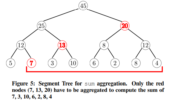
正如我们在上一节中看到的，即使是可移除的累积算法也会导致二次方执行时间，因为当窗口帧对于每个元组任意更改时，缓存上一个窗口的结果没有帮助。因此，我们引入了一个额外的数据结构，线段树，它允许对O（logn）中任意帧上的聚合求值。在图中，sum用作聚合，因此根节点存储所有叶的和节点根的两个子级存储两个等宽子范围的和，依此类推。分段树可以利用聚合的结合性，在对数时间内计算任意范围内的聚合。例如，要计算序列最后7个值的和，我们需要计算红色节点7、13和20的和。

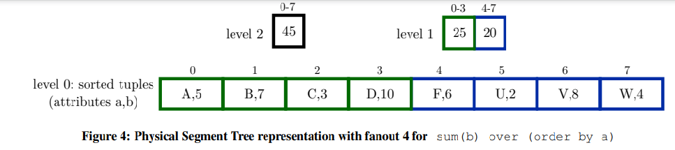
For illustration purposes, Figure 5 shows the Segment Tree as a binary tree with pointers. In fact, our implementation stores all nodes of each tree level in an array and without any pointers, as shown in Figure 4. In this compact representation, which is similar to that of a standard binary heap, the tree structure is implicit and the child and parent of a node can be determined using arithmetic operations. Furthermore, to save even more space, the lowest level of the tree is the sorted input data itself, and we use a larger fanout (4 in the figure). These optimizations make the additional space consumption for the Segment Tree negligible. Additionally, the higher fanout improves performance, as we show in an experiment that is described in Section 5.7.

为了便于说明，图5将段树显示为带指针的二叉树。实际上，我们的实现将每个树级别的所有节点存储在一个数组中，没有任何指针，如图4所示。在这种与标准二进制堆类似的紧凑表示中，树结构是隐式的，并且可以使用算术运算确定节点的子节点和父节点。此外，为了节省更多空间，树的最低层是已排序的输入数据本身，我们使用更大的扇形分叉（图中为4）。这些优化使得段树的额外空间消耗可以忽略不计。另外，在第5.7节中，我们还描述了一个更高的性能。

In order to compute an aggregate for a given range, the Segment Tree is traversed bottom up starting from both window frame bounds. Both traversals are done simultaneously until the traversals arrive at the same node. As a result, this procedure stops early for small ranges and always aggregates the minimum number of nodes.The details of the traversal algorithm can be found in Appendix C.

为了计算给定范围的聚合，线段树从两个窗口帧边界开始自下而上遍历。两边遍历同时进行，直到遍历到达同一个节点。因此，此过程在小范围内提前停止，并始终聚集最小数量的节点。遍历算法的细节可以在附录C中找到。

In addition to improving worst-case efficiency, another important benefit of the Segment Tree is that it allows to parallelize arbitrary aggregates, even for running sum queries like sum(b) over (order by a rows between unbounded preceding and current row). This is particularly important for queries without a partitioning clause, which can only use intra-partition parallelism to avoid executing this phase of the algorithm serially. The Segment Tree itself can easily be constructed in parallel and without any synchronization,in a bottom-up fashion: All available threads scan adjacent ranges of the same Segment Tree level (e.g., using a parallel for construct) and store the computed aggregates into the level above it.

除了提高最坏情况下的效率外，线段树的另一个重要好处是，它允许并行化任意聚合，甚至可以在sum（b）over（order by a rows between unbounded preceding and current row）等sum查询。这对于没有分区子句的查询尤其重要，因为分区子句只能使用分区内并行来避免算法的这一阶段的串行执行。线段树本身可以很容易地以自底向上的方式并行构造，而无需任何同步：所有可用线程扫描同一线段树级别的相邻范围（例如，使用parallel for construct），并将计算的聚合存储到它上面的级别中。

For aggregate functions like min, max, count, and sum, the Segment Tree uses the obvious corresponding aggregate function. For derived aggregate functions like avg or stddev, it is more efficient to store all needed values (e.g., the sum and the count) in the same Segment Tree instead of having two such trees. Interestingly, besides for computing aggregates, the Segment Tree is also useful for parallelizing the dense rank function, which computes a rank without gaps. To compute the dense rank of a particular tuple, the number of distinct values that precede this tuple must be known. A Segment Tree where each segment counts the number of distinct child values is easy to construct , and allows threads to work in parallel on different ranges of the partition.

对于聚合函数，如min、max、count和sum，线段树使用明显对应的聚合函数。对于派生的聚合函数，如avg或stddev，将所有需要的值（例如sum和count）存储在同一线段树中，而不是有两个这样的树，效率更高。有趣的是，除了用于计算聚合外，线段树还可用于并行化dense rank函数，该函数用于计算无间隙排名。要计算特定元组的dense rank，必须知道该元组之前的不同值的数目。在线段树中，每个段都计算不同子值的数量，这很容易构造，并允许线程在分区的不同范围内并行工作。

Algorithm Choice算法选择

Table 1 summarizes the worst-case complexities of the 4 algorithms. The naive algorithm results in quadratic runtime for many common window function queries. The cumulative algorithm works well as long as the window frame only grows. Additionally, queries with frames like current row and unbounded following or 1 preceding and unbounded following can also be executed efficiently using the cumulative algorithm by first reversing the sort order. The removable algorithm further expands the set of queries that can be executed efficiently, but requires an additional ordered tree structure for min and max aggregates and can still result in quadratic runtime if the frame bounds are not constant.

 

 

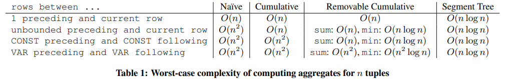
 表1总结了4种算法的最坏情况下的复杂性。对于许多常见的窗口函数查询，简单算法会导致二次方运行时。只要窗口帧只增长，累积算法就可以很好地工作。此外，通过首先反转排序顺序，还可以使用累积算法高效地执行具有诸如current row and unbounded following或1 previous and unbounded following之类的帧的查询。可移动累积算法进一步扩展了可以高效执行的查询集，但是对于最小和最大聚合，需要一个额外的有序树结构，并且如果帧边界不是常数，则仍然可以产生二次方运行时间。

Therefore, the analysis might suggest that the Segment Tree algorithm should always be chosen, as it avoids quadratic runtime in all cases. However, for many simple queries like rows between 1 preceding and current row, the simpler algorithms perform better in practice because the Segment Tree can incur a significant overhead both for constructing and traversing the tree structure. Intuitively, the Segment Tree approach is only beneficial if the frame frequently changes by a large amount in comparison with the previous tuple’s frame. Unfortunately, in many cases, the optimal algorithm cannot be chosen based on the query structure alone, because the data distribution determines whether building a Segment Tree will pay off. Furthermore, choosing the optimal algorithm becomes even more difficult when one also considers parallelism, because, as mentioned before, the Segment Tree algorithm always scales well in the intra-partition parallelism case whereas the other algorithms do not.

因此，以上分析可能建议始终选择线段树算法，因为它在所有情况下都避免了二次方运行时间。然而，对于许多简单的查询，比如rows between 1 preceding and current row，更简单的算法在实际中表现更好，因为线段树在构造和遍历树结构时都会产生很大的开销。直观地说，线段树方法只在帧与前一个元组的帧相比频繁地变化时才有用。不幸的是，在许多情况下，不能仅仅根据查询结构来选择最佳算法，因为数据分布决定了构建一个线段树是否是值得的。此外，当同时考虑并行性时，选择最优算法变得更加困难，因为如前所述，线段树算法在分区内并行情况下总是能够很好地伸缩，而其他算法则不然。

Fortunately, we have found that the majority of the overall query time is spent in the partitioning and sorting phases (cf. Figure 2 and Figure 10), thus erring on the side of the Segment Tree is always a safe choice. We therefore propose an opportunistic approach: A simple algorithm like cumulative aggregation is only chosen when there is no risk of O(n2) runtime and no risk of insufficient parallelism. This method only uses the static query structure, and does not rely on cardinality estimates from the query optimizer.A query like sum(b) over (order by a rows between unbounded preceding and current row), for example, can always safely and efficiently be evaluated using the cumulative algorithm. Additionally, we choose the algorithm for interpartition parallelism and the intra-partition parallelism hash groups separately. For example, the small hash groups of a query might use the cumulative algorithm, whereas the large hash groups might be evaluated using the Segment Tree to make sure evaluation scales well. This approach always avoids quadratic runtime, scales well on systems with many cores, while achieving optimal performance for many common queries.

幸运的是，我们发现大部分查询时间都花在分区和排序阶段（参见图2和图10），因此在线段树的一侧出错总是一个安全的选择。因此，我们提出了一种机会主义的方法：只有在不存在O（n2）运行风险和低效的并行时，才会选择像累积聚合这样的简单算法。此方法只使用静态查询结构，不依赖查询优化器的基数估计。例如，sum（b）over（order by a rows between unbounded preceding and current row）之类的查询总是可以使用累积算法安全高效地进行计算。另外，我们分别选择了分区间并行算法和分区内并行Hash组算法。例如，一个查询的小Hash组可以使用累积算法，而大的Hash组可以使用线段树进行求值，以确保求值具有良好的伸缩性。这种方法总是避免二次方运行时间，在具有多个核心的系统上可以很好地扩展，同时为许多常见查询实现最佳性能。

Window Functions without Framing不带帧的window函数

Window functions that are not affected by framing are less complicated than aggregates as they do not require any complex aggregation algorithms and do not need to compute the window frame.Nevertheless, the high-level structure is similar due to supporting intra-partition parallelism and the need to compute partition boundaries. Generally, the implementation on window functions that are not affected by framing consists of two steps: In the first step, the result for the first tuple in the work range is computed. In the second step, the remaining results are computed sequentially by using the previously computed result.

不受帧影响的窗口函数比聚合函数复杂，因为它们不需要任何复杂的聚合算法，也不需要计算窗口帧。不过，由于支持分区内并行和需要计算分区边界，因此高层结构类似。一般来说，不受帧影响的窗口函数的实现包括两个步骤：第一步，计算工作范围内第一个元组的结果。在第二步中，使用先前计算的结果按顺序计算剩余结果。

 

Figure 6 shows the pseudo code of the rank function, which we use as an example. Most of the remaining functions have a similar structure and are shown in Appendix D. To compute the rank of an arbitrary tuple at index begin, the index of the first peer is computed using binary search (done by findFirstPeer in line 5). All tuples that are in the same partition and have the same order by key(s) are considered peers. Given this first result, all remaining rank computations can then assume that the previous rank has been computed (lines 10-13). All window functions without framing are quite cheap to compute, since they consist of a sequential scan that only looks at neighboring tuples.

 

 

 

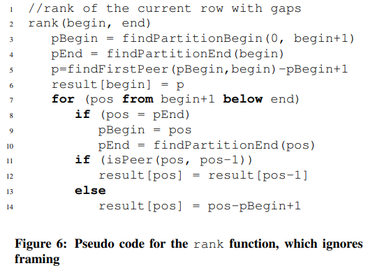
图6显示了rank函数的伪代码，我们用它作为示例。其余的大多数函数都有类似的结构，如附录D所示。要计算索引开始时任意元组的rank，使用折半查找（由findFirstPeer在第5行中完成）计算第一个对等元组的索引。所有在同一分区中且键顺序相同的元组都被视为对等元组。考虑到第一个结果，所有剩余的rank计算都可以假设先前的rank已经被计算出来（第10-13行）。所有没有帧的窗口函数的计算成本都很低，因为它们由一个只查看相邻元组的顺序扫描组成。

Database Engine Integration数据库引擎集成

Our window function algorithm can be integrated into different database query engines, including query engines that use the traditional tuple-at-a-time model (Volcano iterator model), vector ata-time execution [11], or push-based query compilation [19]. Of course, the code structure heavily depends on the specific query engine. The pseudo code in Figure 6 is very similar to the code generated by our implementation, which is integrated into HyPer and uses push-based query compilation.

我们的窗口函数算法可以集成到不同的数据库查询引擎中，包括使用传统tuple-at-a-time模型（火山迭代器模型）、向量ata-time执行[11]或基于推送的查询编译[19]的查询引擎。当然，代码结构很大程度上依赖于特定的查询引擎。图6中的伪代码与我们的实现生成的代码非常相似，它被集成到HyPer中并使用基于推送的查询编译。

The main difference is that in our implementation and in contrast to the pseudo code shown, we do not store the computed result in a vector (lines 6,12,14), but directly push the tuple to the next operator. This is both faster and uses less space. Also note that, regardless of the execution model, the window function operator is a full pipeline breaker, i.e., it must consume all input tuples before it can produce results. Only during the final window function evaluation phase, can tuples be produced on the fly.

主要区别在于，在我们的实现中，与所示的伪代码相比，我们不将计算结果存储在向量中（第6、12、14行），而是直接将元组推送到下一个算子。这既快又占用空间少。还要注意，不管执行模型是什么，window函数操作符都是一个完整的管道中断器，也就是说，在产生结果之前，它必须消耗所有的输入元组。只有在最后的窗口函数求值阶段，才能动态生成元组。

The parallelization strategy described in Section 3 also fits into HyPer’s parallel execution framework [17], which breaks up work into constant-sized work units (“morsels”). These morsels are scheduled dynamically using work stealing, which allows to distribute work evenly between the cores and to quickly react to workload changes. The morsel-driven approach can be used for the initial partitioning and copying phases, as well as the final window function computation phase.

第3节描述的并行化策略也适用于HyPer的并行执行框架[17]，该框架将工作分解为固定大小的工作单元（“morsels”）。这些信息是使用工作窃取动态调度的，这样可以在核心之间均匀地分配工作，并对工作负载变化做出快速反应。morsel驱动的方法可以用于初始分割和复制阶段，以及最终的窗口函数计算阶段。

 Multiple Window Function Expressions多窗口函数表达式

For simplicity of presentation, we have so far assumed that the query contains only one window function expression. Queries that contain multiple window function expressions, can be computed by adding successive window operators for each expression. HyPer currently uses this approach, which is simple and general but wastes optimization opportunities for queries where the partitioning and ordering clauses are shared between multiple window expressions. Since partitioning and sorting usually dominate the overall query execution time, avoiding these phases can be very beneficial.

为了简化表示，到目前为止，我们假设查询只包含一个窗口函数表达式。包含多个窗口函数表达式的查询，可以通过为每个表达式添加连续的窗口运算符来计算。HyPer目前使用这种方法，这种方法简单而通用，但是对于在多个窗口表达式之间共享分区和排序子句的查询，会浪费优化机会。由于分区和排序通常支配整个查询执行时间，因此避免这些阶段可能非常有益。
Cao et al. [12] discuss optimizations that avoid unnecessary partitioning and sorting steps in great detail. In our compilation based query engine, the final evaluation phase (as shown in Figure 6),could directly compute all window expressions with shared partitioning/ordering clauses. We plan to incorporate this feature into HyPer in the future.

曹等。[12] 详细讨论避免不必要的分区和排序步骤的优化。在我们基于编译的查询引擎中，最后的求值阶段（如图6所示）可以直接使用共享分区/排序子句计算所有窗口表达式。我们计划将来将此功能并入HyPer。