详细介绍：线性代数 · 矩阵 | 四个基本子空间与相关分解

注：英文引文，机翻未校。
如有内容异常，请看原文。

---

The Four Fundamental Subspaces: 4 Lines

四个基本子空间：四条线

Gilbert Strang, Massachusetts Institute of Technology
吉尔伯特·斯特朗，麻省理工学院

1. Introduction

1. 引言
The expression “Four Fundamental Subspaces” has become familiar to thousands of linear algebra students. Those subspaces are the column space and the nullspace of$A$ and $A^T$. They lift the understanding of$Ax=b$to a higher level—a subspace level. The first step sees$Ax$(matrix times vector) as a combination of the columns of$A$. Those vectors$Ax$fill the column space$C(A)$. When we move from one combination to all combinations (by allowing every$x$), a subspace appears.$Ax=b$has a solution exactly when$b$is in the column space of$A$.
“四个核心子空间”这一表述已为成千上万的线性代数学习者所熟知。这些子空间包括矩阵$A$及其转置矩阵$A^T$的列空间与零空间。它们将对$Ax=b$的理解提升到了一个更高的层次——子空间层次。第一步，我们将$Ax$（矩阵与向量的乘积）视为矩阵$A$各列的线性组合，所有这样的向量$Ax$构成了列空间$C(A)$。当大家从单一组合扩展到所有可能的组合（即允许$x$取任意值）时，子空间便随之形成。方程$Ax=b$有解的充要条件是向量$b$ 属于矩阵 $A$ 的列空间。

The next section of this note will introduce all four subspaces. They are connected by the Fundamental Theorem of Linear Algebra. A perceptive reader may recognize the Singular Value Decomposition, when Part 3 of this theorem provides perfect bases for the four subspaces. The three parts are well separated in a linear algebra course! The first part goes as far as the dimensions of the subspaces, using the rank. The second part is their orthogonality—two subspaces in$R^n$and two in$R^m$. The third part needs eigenvalues and eigenvectors of$A^{T}A$to find the best bases. Figure 1 will show the “big picture” of linear algebra, with the four bases added in Figure 2.
本文的下一节将介绍全部四个子空间。它们通过线性代数基本定理相互关联。细心的读者可能会意识到，当该定理的第三部分为这四个子空间提供完美的基时，这便与奇异值分解有所呼应。这三个部分在线性代数课程中是彼此独立但又逐步深入的！第一部分侧重于利用秩来确定子空间的维度。第二部分探讨它们的正交性——即$R^n$中的两个子空间和$R^m$中的两个子空间之间的关系。第三部分则需要借助$A^{T}A$的特征值和特征向量来确定最佳基。图 1 将展示线性代数的“全貌”，而图 2 将在其中加入四个基的示意图。

The main purpose of this paper is to see that theorem in action. We choose a matrix of rank one. When$m=n=2$, all four fundamental subspaces are lines in$R^2$. The big picture is particularly clear, and some would say the four lines are trivial. But the angle between$x$ and $y$decides the eigenvalues of$A$and its Jordan form—those go beyond the Fundamental Theorem. We are seeing the orthogonal geometry that comes from singular vectors and the skew geometry that comes from eigenvectors. One leads to singular values and the other leads to eigenvalues.
本文的核心目的是验证该定理的实际应用。我们选取一个秩为 1 的矩阵，当$m=n=2$时，四个基本子空间均为$R^2$中的直线。此时整体框架尤为清晰，有些人可能会认为这四条直线过于轻松。但向量$x$ 与 $y$之间的夹角决定了矩阵$A$的特征值及其若尔当（Jordan）标准形，而这些内容已超出了线性代数基本定理的范畴。我们将看到由奇异向量构建的正交几何结构，以及由特征向量构建的非对称几何结构：前者对应奇异值，后者对应特征值。

Examples are amazingly powerful. I hope this family of 2 by 2 matrices fills a space between working with a specific numerical example and an arbitrary matrix.
实例具有极强的说服力。希望这类 2×2 矩阵能填补“具体数值实例”与“任意矩阵”之间的研究空白。

2. The Four Subspaces

2. 四个基本子空间
Figure 1 shows the fundamental subspaces for an$m$ by $n$matrix of rank$r$. It is useful to fix ideas with a 3 by 4 matrix of rank 2:
图 1 展示了秩为$r$ 的 $m\times n$矩阵所对应的四个基本子空间。为便于理解，我们选取一个秩为 2 的 3×4 矩阵作为实例：
$$A=\left[\begin{array}{llll}1& 0& 2& 3\\ 0& 1& 4& 5\\ 0& 0& 0& 0\end{array}\right]$$

That matrix is in row reduced echelon form and it shows what elimination can accomplish. The column space of$A$and the nullspace of$A^T$have very simple bases:
该矩阵已化为行最简阶梯形，直观体现了矩阵消元所能达到的效果。矩阵$A$ 的列空间 $C(A)$ 与 $A^T$ 的零空间 $N(A^T)$具有非常简单的基：
$$\left[\begin{array}{l}1\\ 0\\ 0\end{array}\right]\text{and}\left[\begin{array}{l}0\\ 1\\ 0\end{array}\right]\text{span}C(A),\left[\begin{array}{l}0\\ 0\\ 1\end{array}\right]\text{spans}N(A^T).$$

After transposing, the first two rows of$A$are a basis for the row space—and they also tell us a basis for the nullspace:
对矩阵 $A$转置后，其前两行构成行空间的一组基，同时大家也能由此得到零空间的一组基：
$$\left[\begin{array}{l}1\\ 0\\ 2\\ 3\end{array}\right]\text{and}\left[\begin{array}{l}0\\ 1\\ 4\\ 5\end{array}\right]\text{span}C(A^T),\left[\begin{array}{r}-2\\ -4\\ 1\\ 0\end{array}\right]\text{and}\left[\begin{array}{r}-3\\ -5\\ 0\\ 1\end{array}\right]\text{span}N(A).$$

The last two vectors are orthogonal to the first two. But these are not orthogonal bases. Elimination is enough to give Part 1 of the Fundamental Theorem:
后两个向量与前两个向量正交，但它们并非正交基。仅通过矩阵消元，我们就能得到线性代数基本定理的第一部分：
$$\begin{array}{rl}\text{Part 1}& \text{The column space and row space have equal dimension}r=\text{rank}\\ & \text{列空间与行空间的维数相等，均为}r=\text{秩（rank）}\\ & \text{The nullspace}N(A)\text{has dimension}n-r,N(A^T)\text{has dimension}m-r\\ & \text{零空间}N(A)\text{的维数为}n-r，\text{零空间}N(A^T)\text{的维数为}m-r\end{array}$$

That counting of basis vectors is obvious for the row reduced$rref(A)$. This matrix has$r$nonzero rows and$r$pivot columns. The proof of Part 1 is in the reversibility of every elimination step—to confirm that linear independence and dimension are not changed.
对于行最简形矩阵$rref(A)$，基向量的计数是显而易见的：该矩阵具有$r$ 个非零行和 $r$个主元列。第一部分的证明在于每一步消元管理都是可逆的，这确保了线性独立性和（子空间）维数在过程中保持不变。

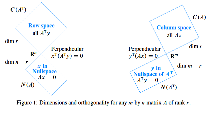
Figure 1: Dimensions and orthogonality for any$m$ by $n$matrix$A$of rank$r$
图 1：秩为$r$ 的任意 $m\times n$ 矩阵 $A$对应的子空间维数与正交关系

Part 2 says that the row space and nullspace are orthogonal complements. The orthogonality comes directly from the equation$Ax=0$. Each$x$in the nullspace is orthogonal to each row:
第二部分指出，行空间与零空间是正交补空间。这种正交性直接源于方程$Ax=0$：零空间中的任意向量$x$都与矩阵的每一行正交，具体推导如下：

$$Ax=0\left[\begin{array}{c}(\text{row 1})\\ \cdots \\ (\text{row}m)\end{array}\right]\left[\begin{array}{c}x\end{array}\right]=\left[\begin{array}{c}0\\ \cdots \\ 0\end{array}\right]\begin{array}{c}\leftarrow x\text{is orthogonal to row 1}\\ \\ \leftarrow x\text{is orthogonal to row}m\end{array}$$

The dimensions of$C(A^T)$ and $N(A)$add to$n$. Every vector in$R^n$is accounted for, by separating$x$ into $x_{\text{row}}+x_{\text{null}}$.
行空间 $C(A^T)$ 与零空间 $N(A)$的维数之和为$n$，因此 $R^n$中的任意向量都可分解为行空间中的分量$x_{\text{row}}$与零空间中的分量$x_{\text{null}}$ 之和，即 $x=x_{\text{row}}+x_{\text{null}}$。

For the 90° angle on the right side of Figure 1, change$A$ to $A^T$. Every vector$b=Ax$in the column space is orthogonal to every solution of$A^{T}y=0$.
对于图 1 右侧所示的 90° 正交关系，只需将矩阵$A$替换为其转置$A^T$即可：列空间中的任意向量$b=Ax$ 都与方程 $A^{T}y=0$的所有解正交。

$$\begin{array}{r}\text{Part 2}C(A^T)=N{(A)}^{\perp }\text{Orthogonal complements正交补空间 in}{R}^n\\ N(A^T)=C{(A)}^{\perp }\text{Orthogonal complements正交补空间 in}{R}^m\end{array}$$

Part 3 of the Fundamental Theorem creates orthonormal bases for the four subspaces. More than that, the matrix is diagonal with respect to those bases$u_1,\dots ,u_n$ and $v_1,\dots ,v_m$. From row space to column space this is$A{v}_i={\sigma }_i{u}_i$ for $i=1,\dots ,r$. The other basis vectors are in the nullspaces:$A{v}_i=0$ and $A^T{u}_i=0$ for $i>r$. When the$u^{\prime }s$ and $v^{\prime }s$are columns of orthogonal matrices$U$ and $V$, we have the Singular Value Decomposition$A=U\Sigma V^T$:
线性代数基础定理的第三部分为四个基本子空间构造了标准正交基。不仅如此，矩阵$A$在这两组基（$u_1,\dots ,u_n$ 和 $v_1,\dots ,v_m$）下可化为对角矩阵。具体而言，从行空间到列空间，对于$i=1,\dots ,r$，有 $A{v}_i={\sigma }_i{u}_i$；而对于 $i>r$，其余基向量分别属于零空间，即$A{v}_i=0$ 且 $A^T{u}_i=0$。当 $u$系列向量构成正交矩阵$U$ 的列、$v$系列向量构成正交矩阵$V$的列时，便得到矩阵的奇异值分解：$A=U\Sigma V^T$，具体形式如下：

$$\text{Part 3}AV=A\left[v_1\cdots v_r\cdots v_n\right]=\left[u_1\cdots u_r\cdots u_m\right]\left[\begin{array}{lll}{\sigma }_1& & \\ & \ddots & \\ & & {\sigma }_r\end{array}\right]=U\Sigma .$$

The $v^{\prime }s$are orthonormal eigenvectors of$A^{T}A$, with eigenvalue${\sigma }_i^2\ge 0$. Then the eigenvector matrix$V$diagonalizes$A^{\text{T}}A=(V{\Sigma }^{\text{T}}{U}^{\text{T}})(U\Sigma V^{\text{T}})=V({\Sigma }^{\text{T}}\Sigma )V^{\text{T}}$. Similarly$U$diagonalizes$A{A}^T$.
其中，$v$系列向量是矩阵$A^{T}A$的标准正交特征向量，对应的特征值为${\sigma }_i^2\ge 0$，因此特征向量矩阵$V$ 可将 $A^{T}A$对角化；同理，$U$ 可将 $A{A}^T$ 对角化。

When matrices are not symmetric or square, it is$A^{T}A$ and $A{A}^T$that make things right.
对于非对称或非方阵而言，正是矩阵$A^{T}A$ 和 $A{A}^T$起到了“修正”作用，使其能够通过奇异值分解转化为对角形式。

This summary is completed by one more matrix: the pseudoinverse. This matrix$A^{+}$inverts$A$where that is possible, from column space back to row space. It has the same nullspace as$A^T$. It gives the shortest solution to$Ax=b$, because$A^{+}b$is the particular solution in the row space:$A{A}^{+}b=b$. Every matrix is invertible from row space to column space, and$A^{+}$provides the inverse:
这部分内容还需补充一个重要矩阵——伪逆（pseudoinverse）。伪逆矩阵$A^{+}$能在可行的范围内实现矩阵$A$的“逆运算”，即从列空间映射回行空间。它与$A^T$具有相同的零空间，并且能给出方程$Ax=b$的最短解（即范数最小的解），因为$A^{+}b$是行空间中的一个特解，满足$A{A}^{+}b=b$。任意矩阵从行空间到列空间的映射都是可逆的，而$A^{+}$正是这一逆映射的体现，具体满足：
$$Pseudoinverse伪逆A^{+}{u}_i=\frac{v_i}{{\sigma }_i}\text{for}i=1,\dots ,r.$$

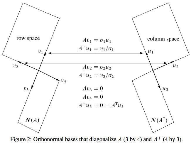
Figure 2: Orthonormal bases that diagonalize$A$(3 by 4) and$A^{+}$(4 by 3)
图 2：使 3×4 矩阵$A$和 4×3 矩阵$A^{+}$对角化的标准正交基

Figure 2 shows the four subspaces with orthonormal bases and the action of$A$ and $A^{+}$. The product$A^{+}A$is the orthogonal projection of$R^n$onto the row space—as near to the identity matrix as possible. Certainly$A^{+}$ is $A^{-1}$when that inverse exists.
图 2 展示了带有标准正交基的四个子空间，以及矩阵$A$ 和伪逆 $A^{+}$的映射作用。乘积$A^{+}A$ 表示 $R^n$最接近单位矩阵的投影矩阵。显然，当矩阵就是到行空间的正交投影，$A$可逆时，其伪逆$A^{+}$就等于其逆矩阵$A^{-1}$。

3. Matrices of Rank One

3. 秩为 1 的矩阵
Our goal is a full understanding of rank one matrices$A=x{y}^T$. The columns of$A$are multiples of$x$, so the column space$C(A)$is a line. The rows of$A$are multiples of$y^T$, so the row space$C(A^T)$is the line through$y$(column vector convention). Let$x$ and $y$be unit vectors to make the scaling attractive. Since all the action concerns those two vectors, we stay in$R^2$:
我们的目标是深入理解秩为 1 的矩阵$A=x{y}^T$。矩阵 $A$的每一列都是向量$x$的倍数，因此其列空间$C(A)$是一条直线；矩阵$A$的每一行都是向量$y^T$的倍数，因此其行空间$C(A^T)$ 是过向量 $y$（按列向量约定）的一条直线。为简化缩放关系，我们设$x$ 和 $y$均为单位向量。由于所有分析仅涉及这两个向量，大家将讨论限定在$R^2$ 空间中：
$$A=x{y}^T=\left[\begin{array}{ll}{x}_1{y}_1& x_1{y}_2\\ x_2{y}_1& x_2{y}_2\end{array}\right].\text{The trace is矩阵的迹为}{x}_1{y}_1+x_2{y}_2=x^{T}y.$$

The nullspace of$A$is the line orthogonal to$y$. It is in the direction of$y^{\perp }$. The algebra gives$A{y}^{\perp }=(x{y}^T)y^{\perp }=0$and the geometry is on the left side of Figure 3. The good basis vectors are$y$ and $y^{\perp }$. On the right side, the bases for the column space of$A$and the nullspace of$A^T$are the orthogonal unit vectors$x$ and $x^{\perp }$.
矩阵 $A$的零空间是与向量$y$正交的直线，方向由$y^{\perp }$（$y$的正交向量）确定。代数上可验证：$A{y}^{\perp }=(x{y}^T)y^{\perp }=0$，其几何意义如图 3 左侧所示，此时理想的基向量为$y$ 和 $y^{\perp }$。图 3 右侧则表明，矩阵$A$ 的列空间与 $A^T$的零空间的基分别为正交单位向量$x$ 和 $x^{\perp }$。

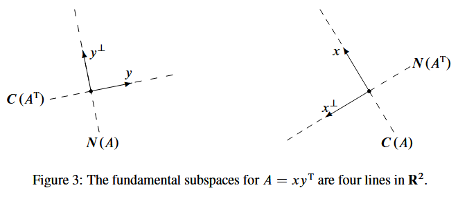
Figure 3: The fundamental subspaces for$A=x{y}^T$are four lines in$R^2$
图 3：矩阵$A=x{y}^T$对应的四个基本子空间是$R^2$中的四条直线

4. Eigenvalues of$x{y}^T$

4. 矩阵 $x{y}^T$ 的特征值
The eigenvalues of$A$were not mentioned in the Fundamental Theorem. Eigenvectors are not normally orthogonal. They belong to the column space and the nullspace, not a natural pair of subspaces. One subspace is in$R^n$, one is in$R^m$, and they are comparable (but usually not orthogonal) only when$m=n$. The eigenvectors of the singular 2 by 2 matrix$A=x{y}^T$ are $x$ and $y^{\perp }$:
线性代数基本定理并未涉及矩阵$A$的特征值。特征向量通常不具有正交性，它们分别属于列空间和零空间，并非自然配对的子空间。这两个子空间一个在$R^n$ 中，一个在 $R^m$ 中，仅当 $m=n$时才可进行比较（但通常仍不正交）。对于奇异的 2×2 矩阵$A=x{y}^T$，其特征向量为$x$ 和 $y^{\perp }$，具体验证如下：
$$Eigenvectors\text{特征向量}Ax=(x{y}^T)x=x(y^{T}x)\text{and 且}A{y}^{\perp }=(x{y}^T)y^{\perp }=0.$$

The new and crucial number is that first eigenvalue${\lambda }_1=y^{T}x=\cos \theta$. This is the trace since${\lambda }_2=0$. The angle$\theta$between row space and column space decides the orientation in Figure 3. The extreme cases$\theta =0$ and $\theta =\pi /2$produce matrices of the best kind and the worst kind:
其中，第一个特征值${\lambda }_1=y^{T}x=\cos \theta$是新的关键参数。由于第二个特征值${\lambda }_2=0$，因此该特征值也等于矩阵的迹。行空间与列空间之间的夹角$\theta$决定了图 3 中的几何方位。当$\theta =0$ 和 $\theta =\pi /2$时，会分别得到“最优”和“最差”类型的矩阵：

• Best: $\cos \theta =1$ when $x=y$. Then$A=x{x}^T$is symmetric with$\lambda =1,0$
  最优情况：当$x=y$ 时，$\cos \theta =1$，此时矩阵 $A=x{x}^T$为对称矩阵，特征值为$\lambda =1,0$

• Worst:$\cos \theta =0$ when $x=y^{\perp }$. Then$A=y^{\perp }{y}^T$has trace zero with$\lambda =0,0$
  最差情况：当$x=y^{\perp }$ 时，$\cos \theta =0$，此时矩阵 $A=y^{\perp }{y}^T$的迹为 0，特征值为$\lambda =0,0$

“Worst” is a short form of “nondiagonalizable”. The eigenvalue$\lambda =0$is repeated and the two eigenvectors$x$ and $y^{\perp }$coincide when the trace$y^{T}x$is zero. At that point$A$cannot be similar to the diagonal matrix of its eigenvalues (because this will be the zero matrix). The right choice of$Q^{-1}AQ$will produce the Jordan form in this extreme case when$x$ and $y$are orthonormal:
“最差”是“不可对角化”的简称。当迹$y^{T}x=0$ 时，特征值 $\lambda =0$为二重特征值，且两个特征向量$x$ 和 $y^{\perp }$重合，此时矩阵$A$无法相似于其特征值构成的对角矩阵（因为该对角矩阵为零矩阵）。在$x$ 和 $y$为标准正交向量的极端情况下，选择合适的矩阵$Q$，可通过 $Q^{-1}AQ$ 将 $A$化为若尔当标准形：
$$J=\left[\begin{array}{l}{x}^T\\ y^T\end{array}\right]\left[\begin{array}{l}x{y}^T\end{array}\right]\left[\begin{array}{ll}x& y\end{array}\right]=\left[\begin{array}{l}{x}^T\\ y^T\end{array}\right]\left[\begin{array}{ll}0& x\end{array}\right]=\left[\begin{array}{ll}0& 1\\ 0& 0\end{array}\right]$$

Jordan chose the best basis ($x$ and $y$) to put$x{y}^T$in that famous form, with an offdiagonal 1 to signal a missing eigenvector. The SVD will choose two different orthonormal bases to put$x{y}^T$in its diagonal form$\Sigma$.
若尔当选择了最优基（$x$ 和 $y$），将矩阵 $x{y}^T$化为上述著名的若尔当标准形，其中非对角元 1 标志着矩阵缺少一个线性无关的特征向量。而奇异值分解（SVD）则会选择两组不同的标准正交基，将$x{y}^T$化为对角矩阵$\Sigma$。

5. Factorizations of$A=x{y}^T$

5. 矩阵 $A=x{y}^T$ 的分解形式

By bringing together three important ways to factor this matrix, you can see the end result of each approach and how that goal is reached. We still have$A=x{y}^T$ and $\text{rank}(A)=1$. The end results are$\Sigma$, $\Lambda$, and $T$.
通过通过整合该矩阵的三种要紧分解方式，我们能够清晰地看到每种方法的最终结果及其实现过程。此处仍设$A=x{y}^T$ 且 $\text{rank}(A)=1$，分解的最终结果分别为对角矩阵$\Sigma$、特征值对角矩阵$\Lambda$和上三角矩阵$T$。

A. Singular Value Decomposition

A. 奇异值分解（SVD）
$$U^{T}AV=\left[\begin{array}{ll}1& 0\\ 0& 0\end{array}\right]=\Sigma$$

B. Diagonalization by eigenvectors

B. 特征向量对角化
$$S^{-1}AS=\left[\begin{array}{cc}\cos \theta & 0\\ 0& 0\end{array}\right]=\Lambda$$

C. Orthogonal triangularization

C. 正交三角化
$$Q^{T}AQ=\left[\begin{array}{cc}\cos \theta & \sin \theta \\ 0& 0\end{array}\right]=T$$

The columns of$U$, $V$, $S$, and $Q$will be$x$, $y$, $y^{\perp }$, and $x^{\perp }$. They come in different orders !
矩阵 $U$、$V$、$S$ 和 $Q$的列向量均为$x$、$y$、$y^{\perp }$ 和 $x^{\perp }$，只是排列顺序不同！

A. In the SVD, the columns of$U$ and $V$are orthonormal bases for the four subspaces. Figure 3 shows$u_1=x$in the column space and$v_1=y$in the row space. Then$Ay=(x{y}^T)y$correctly gives$x$ with ${\sigma }_1=1$. The nullspace bases are$u_2=x^{\perp }$ and $v_2=y^{\perp }$. Notice the different bases in$U$ and $V$, from the reversal of$x$ and $y$:
在奇异值分解中，矩阵 $U$ 和 $V$的列向量分别是四个基本子空间的标准正交基。图 3 显示，$u_1=x$属于列空间，$v_1=y$属于行空间，且$Ay=(x{y}^T)y=x$，对应奇异值${\sigma }_1=1$，这一结果完全正确。零空间的基分别为$u_2=x^{\perp }$（$A^T$零空间的基）和$v_2=y^{\perp }$（$A$零空间的基）。需注意，由于$x$ 和 $y$的“角色反转”，矩阵$U$ 和 $V$中的基向量有所不同，具体推导如下：
$$U^{T}AV={\left[\begin{array}{ll}x& x^{\perp }\end{array}\right]}^T\left[\begin{array}{l}x{y}^T\end{array}\right]\left[\begin{array}{ll}y& y^{\perp }\end{array}\right]={\left[\begin{array}{ll}x& x^{\perp }\end{array}\right]}^T\left[\begin{array}{ll}x& 0\end{array}\right]=\left[\begin{array}{ll}1& 0\\ 0& 0\end{array}\right]=\Sigma$$

The pseudoinverse of$x{y}^T$ is $y{x}^T$. The norm of$A$ is ${\sigma }_1=1$.
矩阵 $x{y}^T$ 的伪逆为 $y{x}^T$，矩阵 $A$的范数等于其最大奇异值，即${\sigma }_1=1$。

B. In diagonalization, the eigenvectors of $A=x{y}^T$ are $x$ and $y^{\perp }$. Those are the columns of the eigenvector matrix$S$, and its determinant is$y^{T}x=\cos \theta$. The eigenvectors of$A^T=y{x}^T$ are $y$ and $x^{\perp }$, which go into the rows of$S^{-1}$(after division by$\cos \theta$):
在特征向量对角化中，矩阵 $A=x{y}^T$的特征向量为$x$ 和 $y^{\perp }$，它们构成特征向量矩阵$S$ 的列，且 $S$ 的行列式为 $y^{T}x=\cos \theta$。矩阵 $A^T=y{x}^T$的特征向量为$y$ 和 $x^{\perp }$，这些向量在除以$\cos \theta$后，构成逆矩阵$S^{-1}$的行，具体推导如下：
$$S^{-1}AS=\frac{1}{\cos \theta }{\left[\begin{array}{ll}y& x^{\perp }\end{array}\right]}^T\left[\begin{array}{l}x{y}^T\end{array}\right]\left[\begin{array}{ll}x& y^{\perp }\end{array}\right]={\left[\begin{array}{ll}y& 0\end{array}\right]}^T\left[\begin{array}{ll}x& 0\end{array}\right]=\left[\begin{array}{cc}\cos \theta & 0\\ 0& 0\end{array}\right]=\Lambda$$

This diagonalization fails when$\cos \theta =0$ and $S$is singular. The Jordan form jumps from$A$ to $J$, as that off-diagonal 1 suddenly appears.
当 $\cos \theta =0$ 时，矩阵 $S$奇异，此时特征向量对角化失效。随着非对角元 1 的突然出现，矩阵形式将从$A$直接“跳跃”到若尔当标准形$J$。

C.One of the many useful discoveries of Isaac Schur is that every square matrix is unitarily similar to atriangular matrix:
：任意方阵都酉相似于一个就是艾萨克·舒尔（Isaac Schur）的众多重要发现之一三角矩阵，即：
$$Q^{\ast }AQ=T\text{with 其中}{Q}^{\ast }Q=I（Q为酉矩阵，实数域中即为正交矩阵）.$$

His construction starts with the unit eigenvector$x$in the first column of$Q$. In our 2 by 2 case, the construction ends immediately with$x^{\perp }$in the second column:
该构造方法的第一步是将单位特征向量$x$ 作为矩阵 $Q$的第一列。在我们所讨论的 2×2 矩阵情形中，构造过程可直接完成——将$x^{\perp }$ 作为 $Q$的第二列，具体推导如下：

$$Q^{T}AQ=\left[\begin{array}{l}{x}^T\\ x^{\perp T}\end{array}\right]\left[\begin{array}{l}x{y}^T\end{array}\right]\left[\begin{array}{lc}x& x^{\perp }\end{array}\right]=\left[\begin{array}{l}{y}^T\\ 0^T\end{array}\right]\left[\begin{array}{ll}x& x^{\perp }\end{array}\right]=\left[\begin{array}{cc}\cos \theta & \sin \theta \\ 0& 0\end{array}\right]=T$$

This triangular matrix$T$still has norm 1, since$Q$is unitary. Numerically$T$is far more stable than the diagonal form$\Lambda$. In fact$T$survives in the limit$\cos \theta =0$of coincident eigenvectors, when it becomes$J$.
由于 $Q$是酉矩阵（实数域中为正交矩阵），三角矩阵$T$的范数仍为 1。从数值计算角度看，$T$远比对角矩阵$\Lambda$稳定。实际上，即使在特征向量重合的极限情况（$\cos \theta =0$）下，$T$依然存在，此时它将退化为若尔当标准形$J$。

Note: The triangular form$T$is not so widely used, but it gives an elementary proof of a seemingly obvious fact: A random small perturbation of any square matrix is almost sure to produce distinct eigenvalues. What is the best proof?
注：三角矩阵 $T$的应用并不广泛，但它为一个看似显而易见的事实提供了简洁证明：对任意方阵进行随机小扰动后，几乎必然会得到具有互异特征值的矩阵。那么，最优的证明方法是什么呢？

More controversially, I wonder if Schur can be regarded as the greatest linear algebraist of all time?
更具争议性的一个挑战是：舒尔是否能被视为有史以来最伟大的线性代数学家？

Summary

总结

The four fundamental subspaces, coming from$A=x{y}^T$and from$A^T=y{x}^T$, are four lines in$R^2$. Their directions are given by$x$, $x^{\perp }$, $y$, and $y^{\perp }$. The eigenvectors of$A$ and $A^T$are the same four vectors. But there is a crucial crossover in the pictures of Figures 1-2-3. The eigenvectors of$A$lie in its column space and nullspace, not a natural pair. The dimensions of the spaces add to$n=2$, but the spaces are not orthogonal and they could even coincide.
由矩阵 $A=x{y}^T$ 及其转置 $A^T=y{x}^T$所确定的四个基本子空间，是$R^2$中的四条直线，其方向分别由向量$x$、$x^{\perp }$、$y$ 和 $y^{\perp }$ 确定。矩阵 $A$ 和 $A^T$的特征向量均为这四个向量，但在图 1-2-3 中存在一个关键的“交叉”现象：矩阵$A$的特征向量分别属于其列空间和零空间，并非自然配对的子空间。尽管这两个子空间的维数之和为$n=2$，但它们并不正交，甚至可能重合。

The better picture is the orthogonal one that leads to the SVD.
更好的图示是那种正交的，它引出了奇异值分解（SVD）。

References

参考文献

These are among the textbooks that present the four subspaces.
以下是部分介绍四个基本子空间的教材：

1. David Lay, Linear Algebra and Its Applications, Third edition, Addison-Wesley (2003).
   戴维·莱（David Lay），《线性代数及其应用》（第三版），Addison-Wesley 出版社（2003 年）。

2. Peter Olver and Chehrzad Shakiban, Applied Linear Algebra, Pearson Prentice-Hall (2006).
   彼得·奥尔弗（Peter Olver）、彻尔扎德·沙基班（Chehrzad Shakiban），《应用线性代数》，Pearson Prentice-Hall 出版社（2006 年）。

3. Theodore Shifrin and Malcolm Adams, Linear Algebra: A Geometric Approach, Freeman (2001).
   西奥多·希夫林（Theodore Shifrin）、马尔科姆·亚当斯（Malcolm Adams），《线性代数：几何方法》，Freeman 出版社（2001 年）。

4. Gilbert Strang, Linear Algebra and Its Applications, Fourth edition, Cengage (previously Brooks/Cole) (2006).
   吉尔伯特·斯特朗（Gilbert Strang），《线性代数及其应用》（第四版），Cengage 出版社（原 Brooks/Cole 出版社）（2006 年）。

5. Gilbert Strang, Introduction to Linear Algebra, Third edition, Wellesley-Cambridge Press (2003).
   吉尔伯特·斯特朗（Gilbert Strang），《线性代数导论》（第三版），Wellesley-Cambridge 出版社（2003 年）。

---

via：

• The Four Fundamental Subspaces: 4 Lines - Gilbert Strang, Massachusetts Institute of Technology
  https://web.mit.edu/18.06/www/Essays/newpaper_ver3.pdf