【循环神经网络2】长短期记忆网络LSTM详解 - 指南

1 LSTM的产生背景

大家首先了解一下长短期记忆网络产生的背景。先回顾一下【循环神经网络1】一文搞定RNN入门与详解-CSDN博客中推导的误差项沿时间反向传播的公式：

我们可以根据下面的不等式，来获取通过的模的上界（模能够看做对中每一项值的大小的度量）：

我们可以看到，误差项从 t 时刻传递到 k 时刻，其值的上界是的指数函数。分别是对角矩阵 和矩阵 模的上界。显然，除非乘积的值位于 1 附近，否则，当 t-k 很大时（也就是误差传递很多个时刻时），整个式子的值就会变得极小（当乘积小于1）或者极大（当乘积大于1），前者就是梯度消失，后者就是梯度爆炸。虽然科学家们搞出了很多技巧（比如怎样初始化权重），让的值尽可能贴近于1，终究还是难以抵挡指数函数的威力。

梯度消失到底意味着什么？在【循环神经网络1】一文搞定RNN入门与详解-CSDN博客中我们已证明，权重数组各个时刻的梯度之和，即：就是最终的梯度

假设从 t-3 时刻开始，梯度已经几乎减少到0了。那么，从这个时刻开始再往之前走，得到的梯度（几乎为零）就不会对最终的梯度值有任何贡献，这就相当于无论 t-3 时刻之前的网络状态 h 是什么，在训练中都不会对权重数组的更新产生影响，也就是网络事实上已经忽略了 t-3 时刻之前的状态。这就是原始RNN无法处理长距离依赖的原因。

既然找到了问题的原因，那么我们就能解决它。从问题的定位到解决，科学家们大概花了7、8年时间。终于有一天，Hochreiter和Schmidhuber两位科学家发明出长短时记忆网络，一举解决这个困难。

---

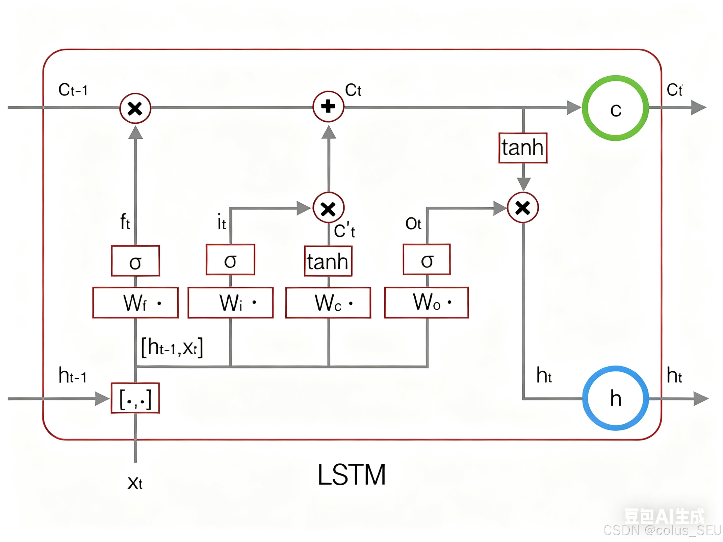
2 LSTM的结构和概念

其实，长短时记忆网络的思路比较简单。原始RNN的隐藏层只有一个状态，即，它对于短期的输入相当敏感。那么，假如我们再增加一个状态，即，让它来保存长期的状态，那么问题不就解决了么？如下图所示：

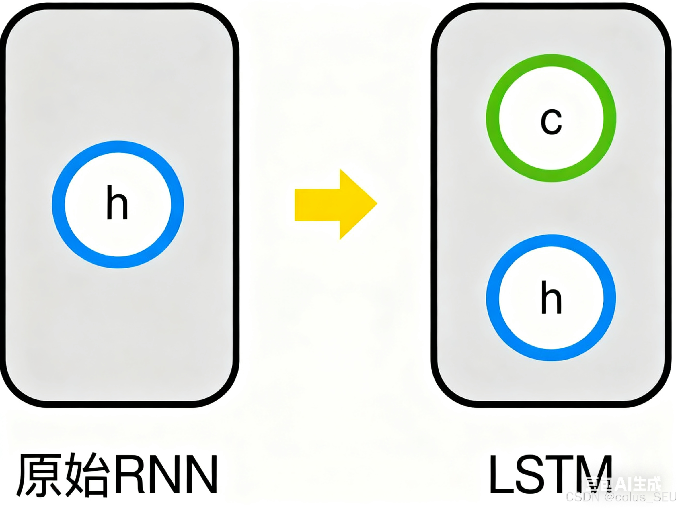
新增加的状态，称为单元状态(cell state)。我们把上图按照时间维度展开：

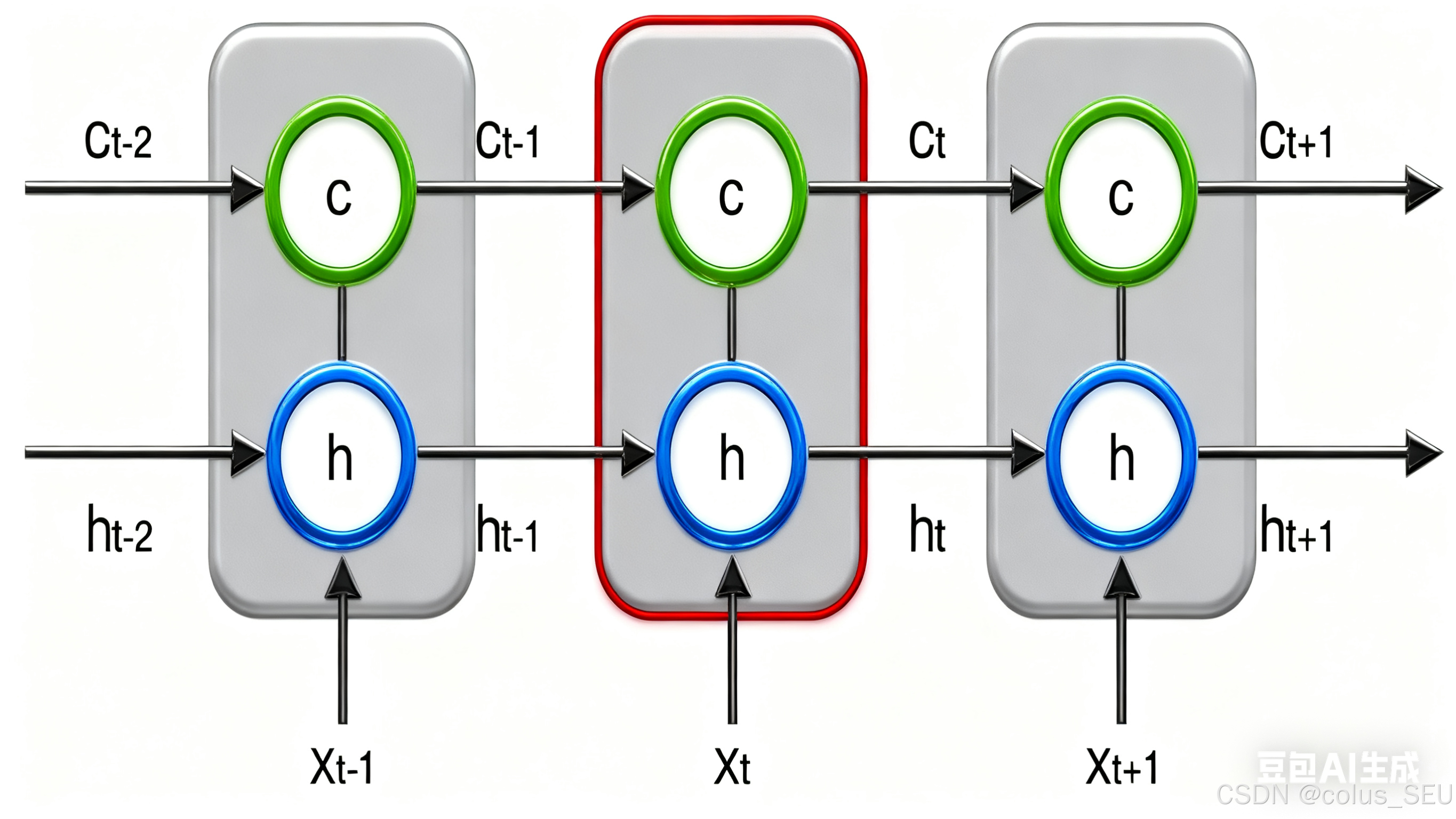
上图仅仅是一个示意图，我们可能看出，在时刻，LSTM的输入有三个：当前时刻网络的输入值、上一时刻LSTM的输出值、以及上一时刻的单元状态；LSTM的输出有两个：当前时刻LSTM输出值、和当前时刻的单元状态。注意 都是向量。

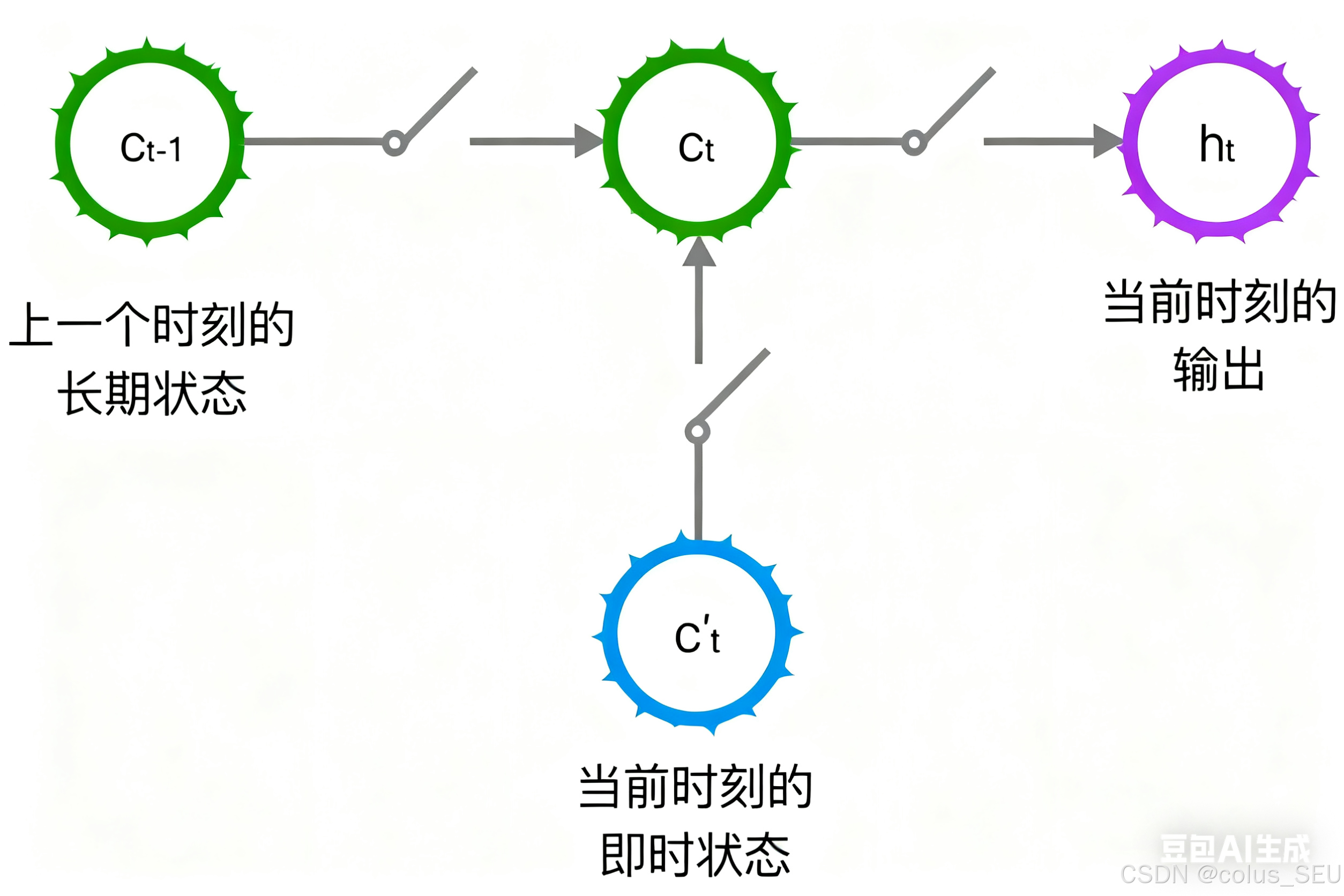
LSTM的关键，就是怎样控制长期状态使用三个控制开关。就是。在这里，LSTM的思路

• 第一个开关，负责控制继续保存长期状态；

• 第二个开关，负责控制把即时状态输入到长期状态；

• 第三个开关，负责控制是否把长期状态作为当前的LSTM的输出。

---

3 LSTM的前向计算

3.1 开关的实现（门）

前面描述的开关是怎样在算法中建立的呢？这就用到了门（gate）一层就是的概念。门实际上就全连接层一个0到1之间的实数向量。假设就是，它的输入是一个向量，输出是门的权重向量，是偏置项，那么门可以表示为：

门的使用，就是用门的输出向量按元素乘以我们需要控制的那个向量。因为门的输出是0到1之间的实数向量，那么，当门输出为0时，任何向量与之相乘都会得到0向量，这就相当于啥都不能通过；输出为1时，任何向量与之相乘都不会有任何改变，这就相当于啥都可以通过。源于（也就是sigmoid函数）的值域是(0,1)，所以门的状态都是半开半闭的。

---

3.2 三种门的介绍

• LSTM用两个门来控制单元状态 的内容：

  • 一个是遗忘门（forget gate），它决定了上一时刻的单元状态有多少保留到当前时刻

  • 另一个是输入门（input gate），它决定了当前时刻网络的输入有多少保存到单元状态

• LSTM用输出门（output gate）来控制单元状态有多少输出到LSTM的当前输出

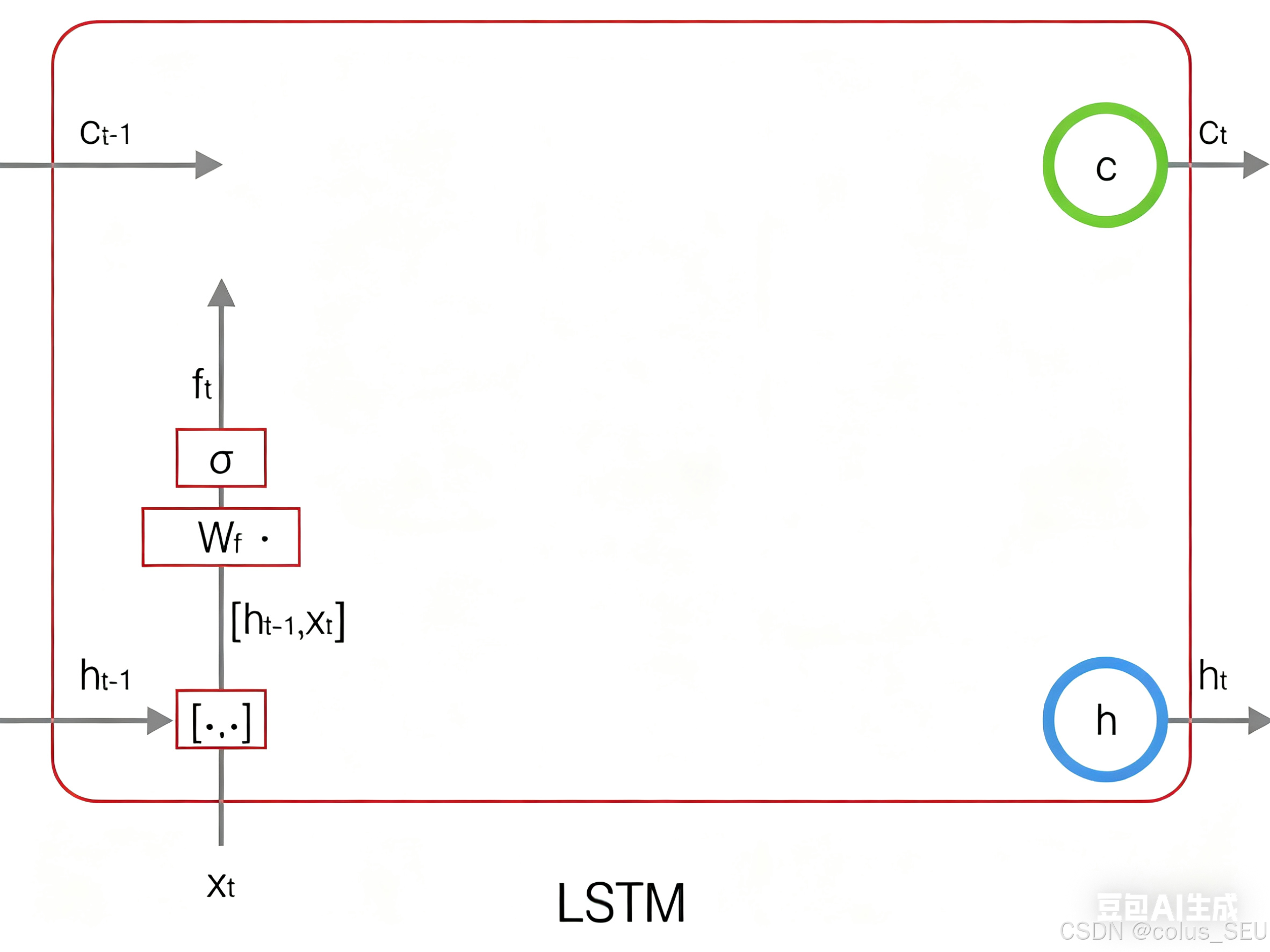
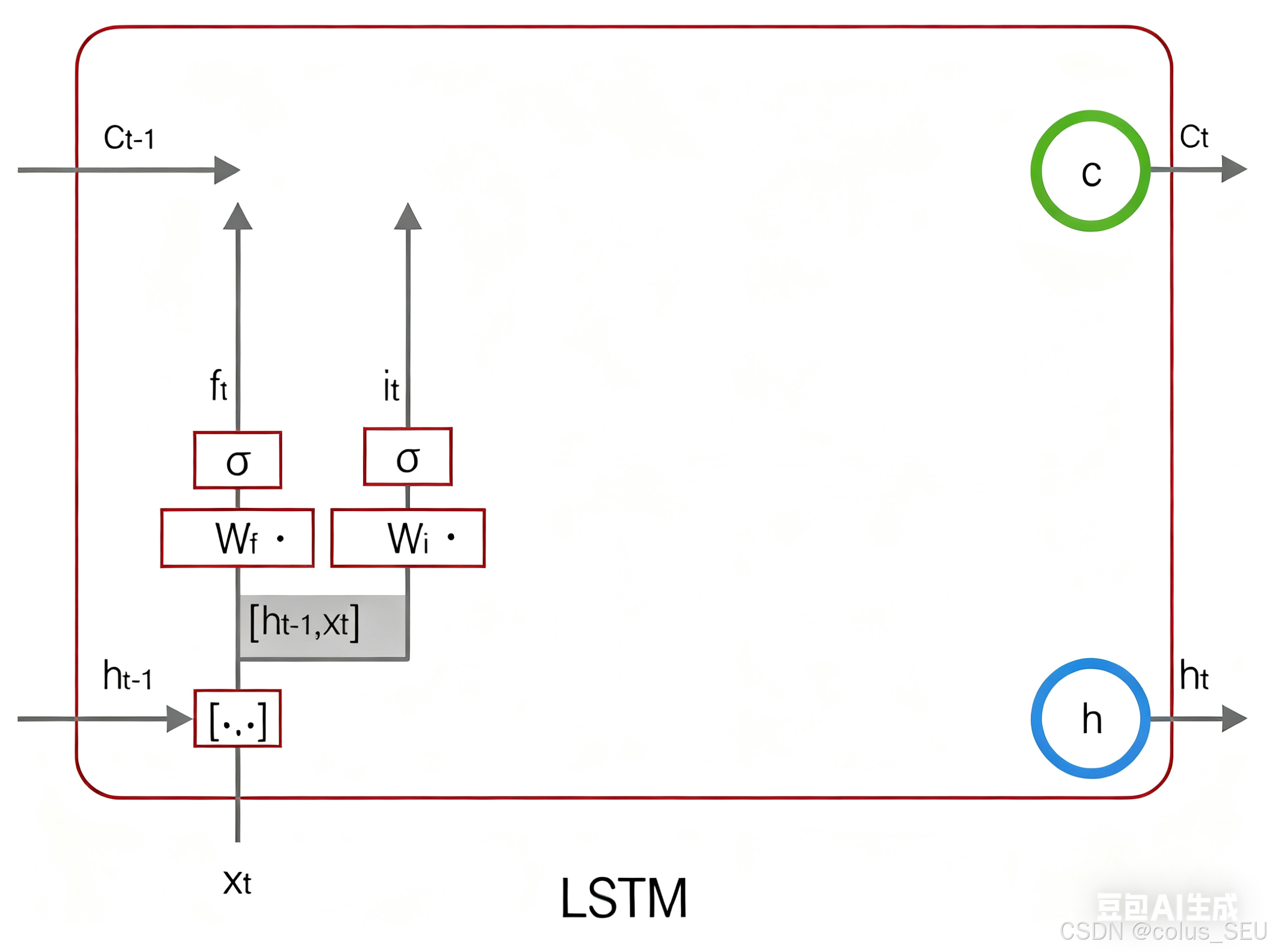
2.3.2.1 遗忘门

• 是遗忘门的权重矩阵

• 表示把两个向量连接成一个更长的向量

• 是遗忘门的偏置项

• 是sigmoid函数

如果输入的维度是，隐藏层的维度是，单元状态的维度是（通常），则遗忘门的权重矩阵 维度是 。事实上，权重矩阵两个矩阵拼接而成的：一个是就是都，它对应着输入项，其维度为 ；一个是 ，它对应着输入项，其维度为。用矩阵分解表示就是：

遗忘门图示如下：

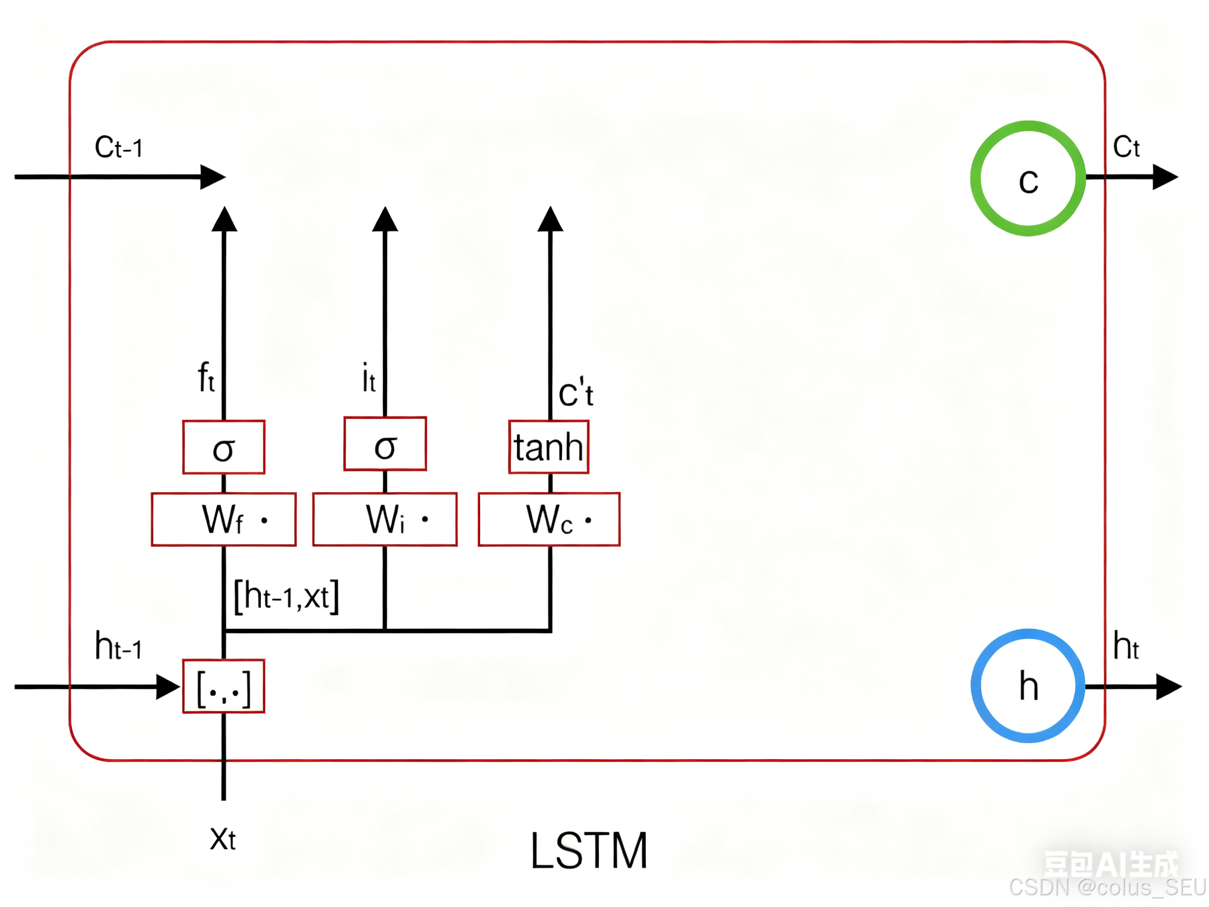
2.3.2.2 输入门：

上式中，是输入门的权重矩阵，是输入门的偏置项。下图表示了输入门的计算：

接下来，我们计算用于描述当前输入的单元状态，它是根据上一次的输出和本次输入来计算的：

下图是 的计算：

现在，我们计算当前时刻的单元状态。它是由上一次的单元状态按元素乘以遗忘门，再用当前输入的单元状态按元素乘以输入门，再将两个积加和产生的：

符号 表示按元素乘。下图是 的计算：

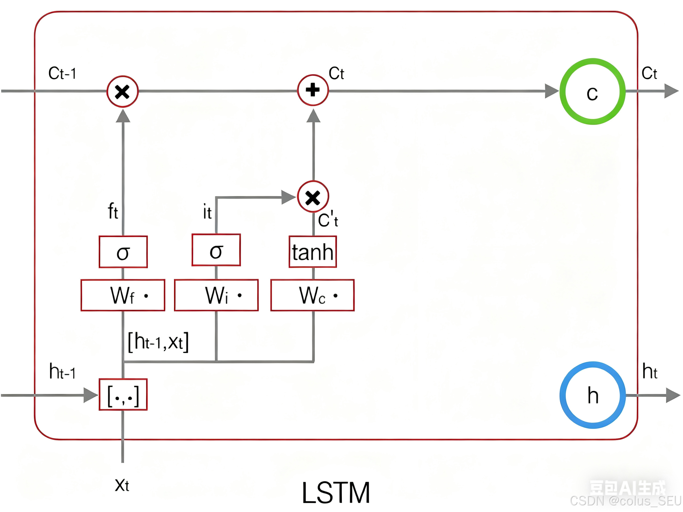
这样，大家就把LSTM关于当前的记忆和长期的记忆组合在一起，形成了新的单元状态。由于遗忘门的控制，它允许保存很久很久之前的信息，由于输入门的控制，它又可以避免当前无关紧要的内容进入记忆。

2.3.2.3 输出门

输出门控制了长期记忆对当前输出的影响：

下图表示输出门的计算：

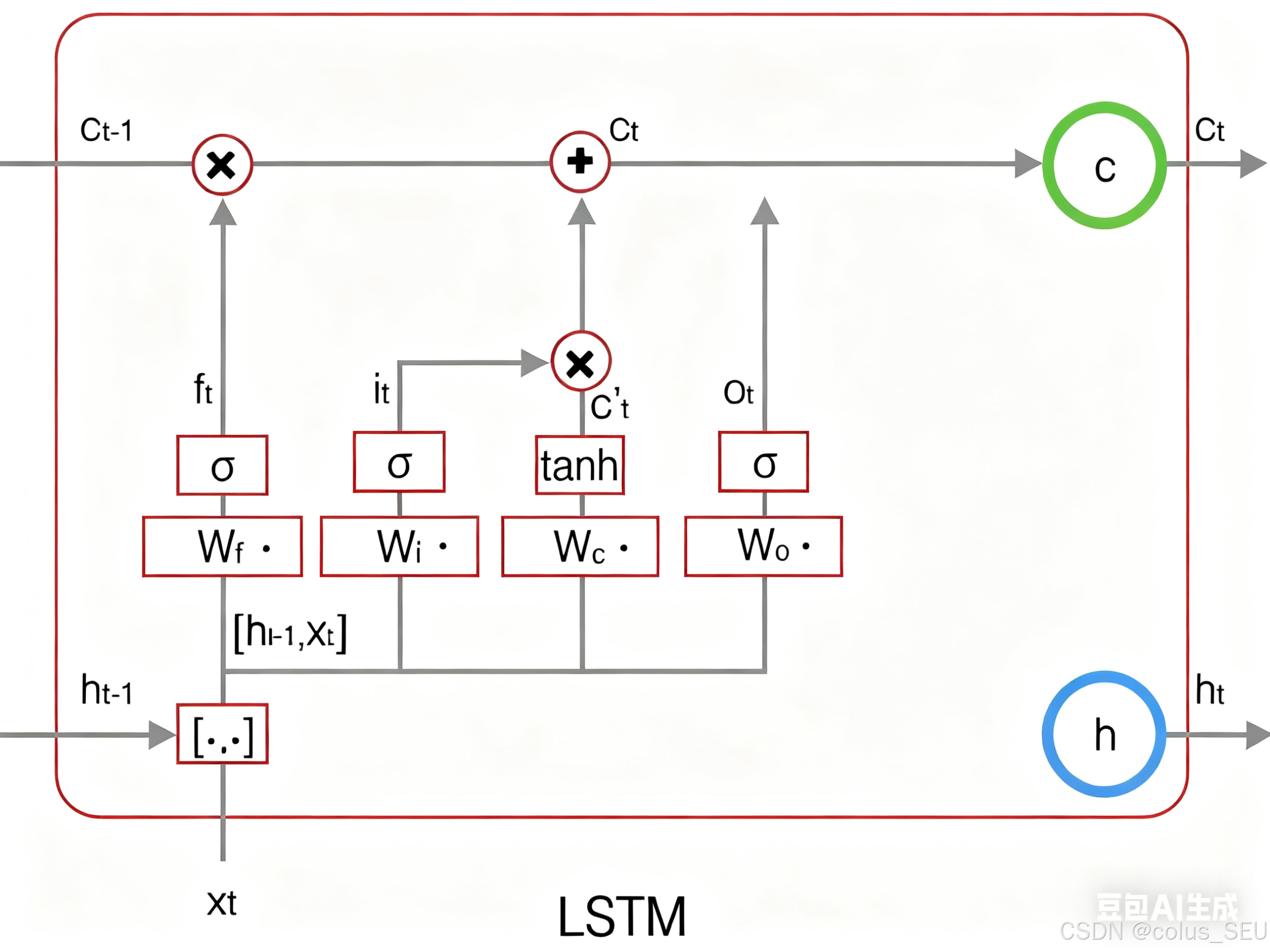
LSTM最终的输出，是由输出门和单元状态共同确定的：

下图表示LSTM最终输出的计算：

式1到式6就是LSTM前向计算的全部公式。

---

4 LSTM的训练

数学公式高能预警！

4.1 LSTM训练算法框架

LSTM的训练仍然使用反向传播算法，

1. 前向计算每个神经元的输出值。对于LSTM来说就是五个向量的值。计算方法已经在上一节中描述过了。

2. 反向计算每个神经元的误差项值。LSTM误差项的反向传播也包括两个方向：

   • 一个是沿时间的反向传播，即从当前时刻开始，计算每个时刻的误差项

   • 一个是将误差项向上一层传播

3. 根据相应的误差项，计算每个权重的梯度。

---

4.2 公式和符号说明

接下来的推导中，我们设定gate的激活函数为sigmoid函数，输出的激活函数为tanh函数：

关于激活函数，以下文章中有具体讲解：

【前馈神经网络详解与实例】2——激活函数_神经网络激活函数例题-CSDN博客https://blog.csdn.net/colus_SEU/article/details/150534855?spm=1001.2014.3001.5501

---

LSTM需要学习的参数共有8组，分别是：遗忘门的权重矩阵 和偏置项 、输入门的权重矩阵 和偏置项 、输出门的权重矩阵 和偏置项 ，以及计算单元状态的权重矩阵 和偏置项 。因为权重矩阵的两部分在反向传播中使用不同的公式，因此在后续的推导中，权重矩阵都将被写为分开的两个矩阵：。

---

我们解释一下按元素乘 符号：

• 当 作用于两个向量时，运算如下：

• 当 作用于一个向量和一个矩阵时，运算如下：

• 当 作用于两个矩阵时，两个矩阵对应位置的元素相乘。

按元素乘可以在某些情况下简化矩阵和向量运算。例如，当一个对角矩阵右乘一个矩阵时，相当于用对角线组成的向量按元素乘那种矩阵：

当一个行向量右乘一个对角矩阵时，相当于该行向量元素乘那个矩阵对角线组成的向量：

上面这两点，在我们后续推导中会多次用到。

---

在 t 时刻，LSTM的输出值为。我们定义 t 时刻的误差项 为：

注意，我们这里假设误差项是损失函数对输出值的导数，而不是对加权输入的导数。因为LSTM有四个加权输入，分别对应四个。但我们仍然需要定义出这四个加权输入，以及他们对应的误差项。就是我们希望往上一层传递一个误差项而不

---

4.3 误差项沿时间的反向传递

沿时间反向传递误差项，就是要计算出t-1时刻的误差项。

我们知道，是一个 Jacobian 矩阵。假设隐藏层 的维度是 的话，那么它就是一个矩阵，因此上述公式需要使用转置。其中的计算公式如下，即前面的式6和式4：

由于 都是 的函数，利用全导数公式可得：

下面，我们要把式7中的每个偏导数都求出来。根据式6，我们许可求出：

根据式4，我们可以求出：

因为：

我们很容易得出：

将上述偏导数带入到式7，我们得到：

根据 的定义，可知：

式8到式12就是将误差沿时间反向传播一个时刻的公式。有了它，大家可以写出将误差项向前传递到任意k时刻的公式：

---

4.4 误差项传递到上一层

大家假设当前为第 层，定义 层的误差项是误差函数对 层加权输入的导数，即：

LSTM的输入由下面的公式计算：

上式中， 表示第 层的激活函数。

因为 都是 的函数， 又是 的函数，因此，要求出 对 的导数，就需使用全导数公式：

式14就是将误差传递到上一层的公式。

---

4.5 权重梯度的计算

对于 的权重梯度，我们知道它的梯度是各个时刻梯度之和（证明过程请参考【循环神经网络1】一文搞定RNN入门与详解-CSDN博客4.3节），我们首先求出它们在时刻的梯度，随后再求出他们的最终的梯度。

我们已经求得了误差项，很容易求出 时刻的：

将各个时刻的梯度加在一起，就能得到最终的梯度：

对于偏置项 的梯度，也是将各个时刻的梯度加在一起。下面是各个时刻的偏置项梯度：

下面是最终的偏置项梯度，即将各个时刻的偏置项梯度加在一起：

对于 的权重梯度，只需要根据相应的误差项直接计算即可：