TensorBoard 简介及使用流程【转】

转自：https://blog.csdn.net/gsww404/article/details/78605784

仅供学习参考，转载地址：http://blog.csdn.net/mzpmzk/article/details/77914941

一、TensorBoard 简介及使用流程

1、TensoBoard 简介

TensorBoard 和 TensorFLow 程序跑在不同的进程中，TensorBoard 会自动读取最新的 TensorFlow 日志文件，并呈现当前 TensorFLow 程序运行的最新状态。

2、TensorBoard 使用流程

添加记录节点：tf.summary.scalar/image/histogram()等

汇总记录节点：merged = tf.summary.merge_all()

运行汇总节点：summary = sess.run(merged)，得到汇总结果

日志书写器实例化：summary_writer = tf.summary.FileWriter(logdir, graph=sess.graph)，实例化的同时传入 graph 将当前计算图写入日志

调用日志书写器实例对象summary_writer的add_summary(summary, global_step=i)方法将所有汇总日志写入文件

调用日志书写器实例对象summary_writer的close()方法写入内存，否则它每隔120s写入一次

二、TensorFlow 可视化分类

1、计算图的可视化：add_graph()

...create a graph...
# Launch the graph in a session.
sess = tf.Session()
# Create a summary writer, add the 'graph' to the event file.
writer = tf.summary.FileWriter(logdir, sess.graph)
writer.close()  # 关闭时写入内存，否则它每隔120s写入一次

2、监控指标的可视化：add_summary()

I、SCALAR

tf.summary.scalar(name, tensor, collections=None, family=None)

可视化训练过程中随着迭代次数准确率(val acc)、损失值(train/test loss)、学习率(learning rate)、每一层的权重和偏置的统计量(mean、std、max/min)等的变化曲线

输入参数：

name：此操作节点的名字，TensorBoard 中绘制的图形的纵轴也将使用此名字

tensor：需要监控的变量 A real numeric Tensor containing a single value.

输出：

A scalar Tensor of type string. Which contains a Summary protobuf.

II、IMAGE

tf.summary.image(name, tensor, max_outputs=3, collections=None, family=None)

可视化当前轮训练使用的训练/测试图片或者 feature maps

输入参数：

name：此操作节点的名字，TensorBoard 中绘制的图形的纵轴也将使用此名字

tensor： A r A 4-D uint8 or float32 Tensor of shape [batch_size, height, width, channels] where channels is 1, 3, or 4

max_outputs：Max number of batch elements to generate images for

输出：

A scalar Tensor of type string. Which contains a Summary protobuf.

III、HISTOGRAM

tf.summary.histogram(name, values, collections=None, family=None)

可视化张量的取值分布

输入参数：

name：此操作节点的名字，TensorBoard 中绘制的图形的纵轴也将使用此名字

tensor： A real numeric Tensor. Any shape. Values to use to build the histogram

输出：

A scalar Tensor of type string. Which contains a Summary protobuf.

IV、MERGE_ALL

tf.summary.merge_all(key=tf.GraphKeys.SUMMARIES)

Merges all summaries collected in the default graph

因为程序中定义的写日志操作比较多，一一调用非常麻烦，所以TensoorFlow 提供了此函数来整理所有的日志生成操作，eg：merged = tf.summary.merge_all ()

此操作不会立即执行，所以，需要明确的运行这个操作(summary = sess.run(merged))来得到汇总结果

最后调用日志书写器实例对象的add_summary(summary, global_step=i)方法将所有汇总日志写入文件

3、多个事件(event)的可视化：add_event()

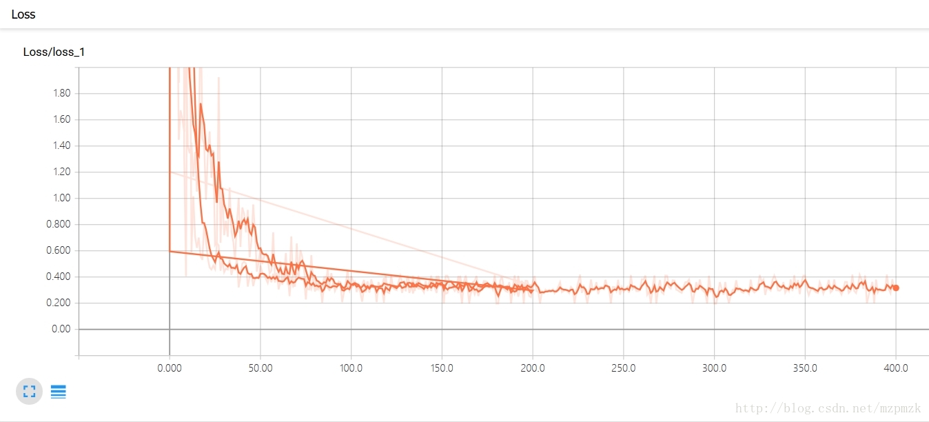
如果 logdir 目录的子目录中包含另一次运行时的数据(多个 event)，那么 TensorBoard 会展示所有运行的数据(主要是scalar)，这样可以用于比较不同参数下模型的效果，调节模型的参数，让其达到最好的效果！

上面那条线是迭代200次的loss曲线图，下面那条是迭代400次的曲线图，程序见最后。

这里写图片描述

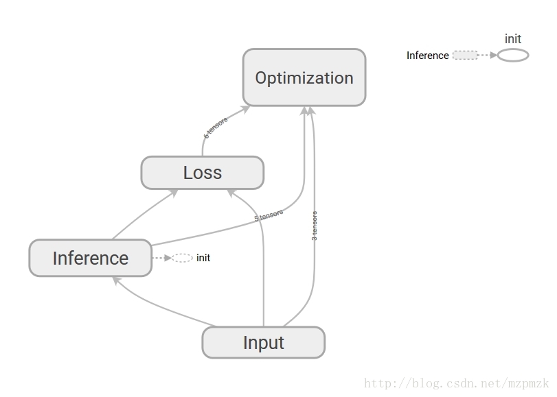
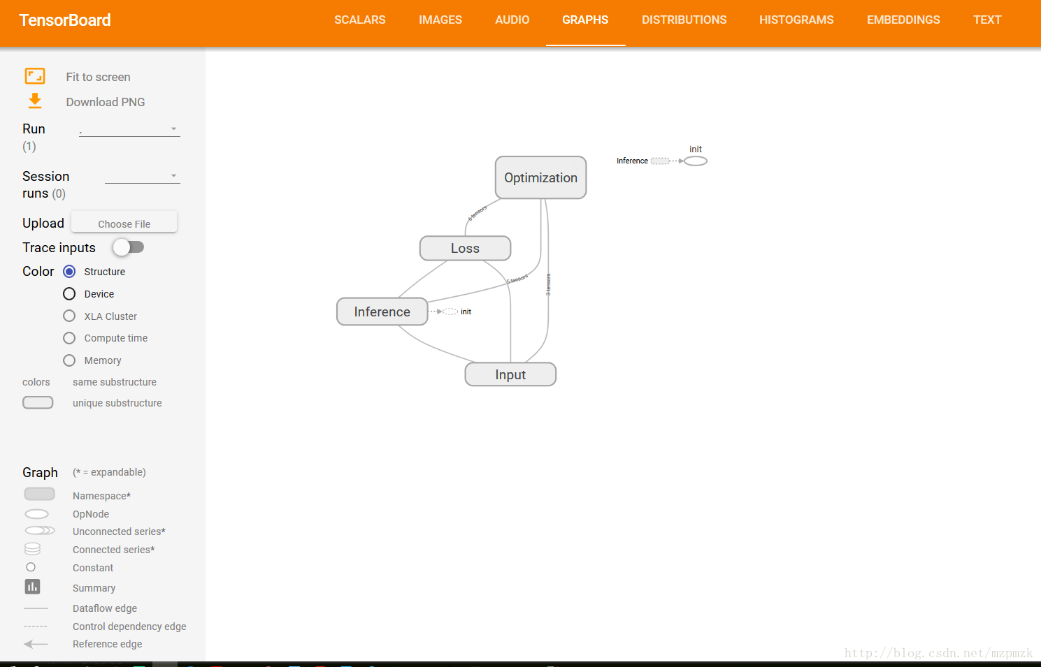
三、通过命名空间美化计算图

使用命名空间使可视化效果图更有层次性，使得神经网络的整体结构不会被过多的细节所淹没

同一个命名空间下的所有节点会被缩略成一个节点，只有顶层命名空间中的节点才会被显示在 TensorBoard 可视化效果图上

可通过tf.name_scope()或者tf.variable_scope()来实现，具体见最后的程序。

这里写图片描述

四、将所有日志写入到文件：tf.summary.FileWriter()

这里写图片描述

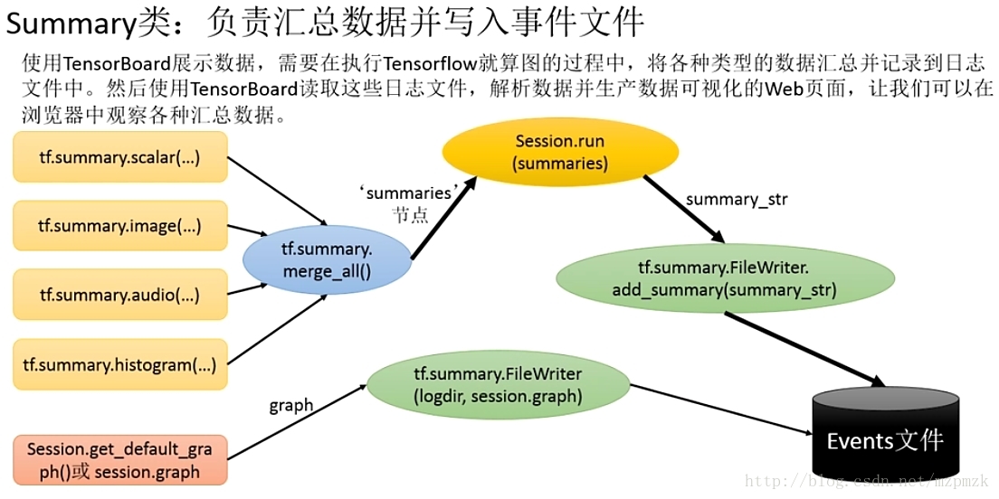
tf.summary.FileWriter(logdir, graph=None, flush_secs=120, max_queue=10)

负责将事件日志(graph、scalar/image/histogram、event)写入到指定的文件中

初始化参数：

logdir：事件写入的目录

graph：如果在初始化的时候传入sess,graph的话，相当于调用add_graph() 方法，用于计算图的可视化

flush_sec：How often, in seconds, to flush the added summaries and events to disk.

max_queue：Maximum number of summaries or events pending to be written to disk before one of the ‘add’ calls block.

其它常用方法：

add_event(event)：Adds an event to the event file

add_graph(graph, global_step=None)：Adds a Graph to the event file，Most users pass a graph in the constructor instead

add_summary(summary, global_step=None)：Adds a Summary protocol buffer to the event file，一定注意要传入 global_step

close()：Flushes the event file to disk and close the file

flush()：Flushes the event file to disk

add_meta_graph(meta_graph_def,global_step=None)

add_run_metadata(run_metadata, tag, global_step=None)

五、启动 TensorBoard 展示所有日志图表

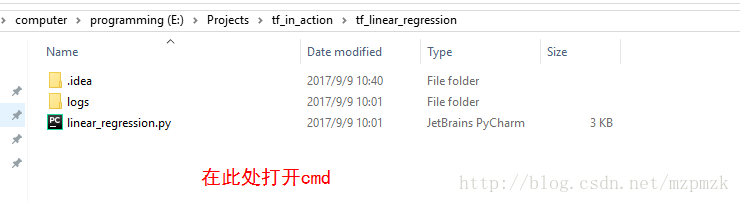
1. 通过 Windows 下的 cmd 启动

运行你的程序，在指定目录下(logs)生成 event 文件
在 logs 所在目录，按住 shift 键，点击右键选择在此处打开 cmd
在 cmd 中，输入以下命令启动 tensorboard --logdir=logs，注意：logs的目录并不需要加引号, logs 中有多个event 时，会生成scalar 的对比图，但 graph 只会展示最新的结果
把下面生成的网址(http://DESKTOP-S2Q1MOS:6006 # 每个人的可能不一样) copy 到浏览器中打开即可

2. 通过 Ubuntu下的 bash 启动

运行你的程序(python my_program.py)，在指定目录下(logs)生成 event 文件
在 bash 中，输入以下命令启动 tensorboard --logdir=logs --port=8888，注意：logs的目录并不需要加引号，端口号必须是事先在路由器中配置好的
把下面生成的网址(http://ubuntu16:8888 # 把ubuntu16 换成服务器的外部ip地址即可) copy 到本地浏览器中打开即可

六、使用 TF 实现一元线性回归(并使用 TensorBoard 可视化)

多个event的loss对比图以及网络结构图(graph)已经在上面展示了，这里就不重复了。

最下面展示了网络的训练过程以及最终拟合效果图

#!/usr/bin/env python3
# -*- coding: utf-8 -*-

import tensorflow as tf
import matplotlib.pyplot as plt
import numpy as np
import os
os.environ['TF_CPP_MIN_LOG_LEVEL'] = '2'


# 准备训练数据，假设其分布大致符合 y = 1.2x + 0.0
n_train_samples = 200
X_train = np.linspace(-5, 5, n_train_samples)
Y_train = 1.2*X_train + np.random.uniform(-1.0, 1.0, n_train_samples)  # 加一点随机扰动


# 准备验证数据，用于验证模型的好坏
n_test_samples = 50
X_test = np.linspace(-5, 5, n_test_samples)
Y_test = 1.2*X_test


# 参数学习算法相关变量设置
learning_rate = 0.01
batch_size = 20
summary_dir = 'logs'

print('~~~~~~~~~~开始设计计算图~~~~~~~~')

# 使用 placeholder 将训练数据/验证数据送入网络进行训练/验证
# shape=None 表示形状由送入的张量的形状来确定
with tf.name_scope('Input'):
    X = tf.placeholder(dtype=tf.float32, shape=None, name='X')
    Y = tf.placeholder(dtype=tf.float32, shape=None, name='Y')


# 决策函数(参数初始化)
with tf.name_scope('Inference'):
    W = tf.Variable(initial_value=tf.truncated_normal(shape=[1]), name='weight')
    b = tf.Variable(initial_value=tf.truncated_normal(shape=[1]), name='bias')
    Y_pred = tf.multiply(X, W) + b


# 损失函数(MSE)
with tf.name_scope('Loss'):
    loss = tf.reduce_mean(tf.square(Y_pred - Y), name='loss')
    tf.summary.scalar('loss', loss)


# 参数学习算法(Mini-batch SGD)
with tf.name_scope('Optimization'):
    optimizer = tf.train.GradientDescentOptimizer(learning_rate).minimize(loss)


# 初始化所有变量
init = tf.global_variables_initializer()


# 汇总记录节点
merge = tf.summary.merge_all()


# 开启会话，进行训练
with tf.Session() as sess:
    sess.run(init)
    summary_writer = tf.summary.FileWriter(logdir=summary_dir, graph=sess.graph)

    for i in range(201):
        j = np.random.randint(0, 10)  # 总共200训练数据，分十份[0, 9]
        X_batch = X_train[batch_size*j: batch_size*(j+1)]
        Y_batch = Y_train[batch_size*j: batch_size*(j+1)]

        _, summary, train_loss, W_pred, b_pred = sess.run([optimizer, merge, loss, W, b], feed_dict={X: X_batch, Y: Y_batch})
        test_loss = sess.run(loss, feed_dict={X: X_test, Y: Y_test})

        # 将所有日志写入文件
        summary_writer.add_summary(summary, global_step=i)
        print('step:{}, losses:{}, test_loss:{}, w_pred:{}, b_pred:{}'.format(i, train_loss, test_loss, W_pred[0], b_pred[0]))

        if i == 200:
            # plot the results
            plt.plot(X_train, Y_train, 'bo', label='Train data')
            plt.plot(X_test, Y_test, 'gx', label='Test data')
            plt.plot(X_train, X_train * W_pred + b_pred, 'r', label='Predicted data')
            plt.legend()
            plt.show()

    summary_writer.close()

这里写图片描述

posted @ 2018-06-22 16:12 Sky&Zhang 阅读(1993) 评论(0) 编辑收藏举报

会员力量，点亮园子希望

刷新页面返回顶部

sky

我所做的事情都是源于自己对梦想的追求--分享技术、共同创造新世界---欢迎交流：zhangbinghua2012@163.com skyzhangbinghua@gmai.com

TensorBoard 简介及使用流程【转】

仅供学习参考，转载地址：http://blog.csdn.net/mzpmzk/article/details/77914941

一、TensorBoard 简介及使用流程

1、TensoBoard 简介

2、TensorBoard 使用流程

二、TensorFlow 可视化分类

1、计算图的可视化：add_graph()

2、监控指标的可视化：add_summary()

I、SCALAR

II、IMAGE

III、HISTOGRAM

IV、MERGE_ALL

3、多个事件(event)的可视化：add_event()

三、通过命名空间美化计算图

四、将所有日志写入到文件：tf.summary.FileWriter()

五、启动 TensorBoard 展示所有日志图表

1. 通过 Windows 下的 cmd 启动

2. 通过 Ubuntu下的 bash 启动

六、使用 TF 实现一元线性回归(并使用 TensorBoard 可视化)

公告