


tensorflow 1.4学习
tensorflow已经更新到2.0版本了,大多数公司还在用1.4的版本,去过了一遍网上tensorflow1.4的教程,记录下。1.4版本的官网教程貌似已下架,主要是api参考:https://github.com/tensorflow/docs/tree/r1.14/site/en/api_docs/python
Tensorflow数据的核心单位是张量 (tensor),就像numpy中的array一样。Tensorflow中还有一个核心知识点就是计算图(computation graph), tensorflow的大多数程序都可以认为包含两部分:
1. 构建计算图
2. 执行计算图
1. 计算图
tensorflow的代码中,有一个默认图概念(default graph),当我们开始一个线程时,tensorflow就会为我们创造一张默认图,在线程中进行的操作(加减乘除),定义的变量和常量,都会被加入到这张默认图中,成为默认图的节点,这个默认图就是常说的计算图,是为了记录各给节点之前的关系,方便tensorflow进行前向的计算和反向的梯度计算。当我们构建完计算图后,需要运行这张图,才能执行图上的操作(即我们定义的加减乘除, 变量赋值等)。如下代码所示:
默认图理解:
import tensorflow as tf
import numpy as np
# tensorflow 创建了一张默认图
# print(tf.get_default_graph())  # 可以获取默认图对象


# 1. 下面的两个matrix常量,和一个矩阵成分操作,会被加入到默认图中
matrix1 = tf.ones(shape=(2, 2), dtype=np.float32)  # 构建一个tensor,值全为1
matrix2 = tf.constant([[1, 2], [3, 4]], dtype=tf.dtypes.float32) # 构建一个常量tensor, 值为[1, 2], [3, 4]
product = tf.matmul(matrix1, matrix2)
# 默认图现在有三个节点, 两个 constant() op, 和一个matmul() op.

# 显示shape,dyupe,没有具体的值
print(matrix1)
print(matrix2)
print(product)


# 2. 创建一个会话session,在session中,可以运行默认图
ses = tf.Session()   # 有一个参数graph, 可以传入需要计算的图,不传参数时,表示默认图


# 3. 在session中计算默认图中的操作
# 调用 sess 的 'run()' 方法来执行矩阵乘法 op, 传入 'product' 作为该方法的参数.
# 'product' 代表了矩阵乘法 op 的输出, 传入它是向方法表明, 我们希望取回矩阵乘法 op 的输出.
# 整个执行过程是自动化的, 会话负责传递 op 所需的全部输入. op 通常是并发执行的.
# 函数调用 'run(product)' 触发了图中三个 op (两个常量 op 和一个矩阵乘法 op) 的执行.
result = ses.run(product)  # 计算product的值,并返回, 注意返回值 'result' 是一个 numpy `ndarray` 对象.

# tensor, 只显示shape,dyupe,没有具体的值
print(matrix1)
print(matrix2)
print(product)

# np.array, 有具体的值
print(result, type(result))


# 4. 关闭session
ses.close()  # 关闭会话

'''
session对象在使用完后需要关闭以释放资源. 除了显式调用 close 外, 也可以使用 “with” 代码块来自动完成关闭动作.

with tf.Session() as sess:
  result = sess.run([product])
  print (result)
'''
2.计算图获取数据和输入数据
上面已经了解到了,可以从计算图中获取计算得到的数据,可以一次性计算和获取多个数据,如下代码中同时获取计算图中两个节点的值:
import tensorflow as tf

matrix1 = tf.constant([[1, 1], [2, 2]])
value1 = tf.constant(3)
value2 = tf.constant(4)

inter_value = tf.add(matrix1, value1)
product = tf.multiply(inter_value, value2)

with tf.Session() as sess:
    result = sess.run([inter_value, product])  #需要获取的多个 tensor 值,在 op 的一次运行中一起获得(而不是逐个去获取 tensor)

  print(result, type(result))  # 输出为两个np.array组成的list; 注意:若run输入的为list,返回结果则为list,

  print(sess.run(product))  # [product]:返回结果则为list; product:返回结果为单个array
上面计算图中,输入的数据都是固定值,我们可以采用占位符来代替这些数据,构建完计算图后,可以通过向计算图中输入数据,从而实习动态数据,如下代码所示:
import tensorflow as tf
import numpy as np

x_value = tf.random.normal((2, 3), 0, 1)
y_value = tf.random.uniform((2, 1), 0, 2)

x = tf.placeholder(dtype=np.float32, shape=(2, 3))
y = tf.placeholder(dtype=np.float32, shape=(2, 1))

weight = tf.constant([[1, 1.5, 0.5]])
bias = tf.constant(0.5)
loss = tf.matmul(x, tf.transpose(weight)) + bias - y

with tf.Session() as sess:
    # 1. 输入数据为np.array类型
    result = sess.run([loss], feed_dict={x: np.array([[1, 2, 3], [4, 5, 6]]),
                                         y: np.array([[1], [2]])})  #np.array数据
    print(result, type(result))

    # 2. 输入数据为list
    result = sess.run([loss], feed_dict={x: [[1, 2, 3], [4, 5, 6]],
                                         y: [[1], [2]]})  # 自动转化为np.array
    print(result, type(result))

    # 3. 输入数据为np.array
    result = sess.run([loss], feed_dict={x: sess.run(x_value),
                                         y: sess.run(y_value)})  # 随机数据
    print(result, type(result))
3. 变量数据
上述数据中涉及到了常量constant,占位符placeholder, tensorflow中还有一种数据:变量Variable。tf.Variable表示的数据,其值时可以更改的,一般用来存储网络的参数,变量在进行计算前,必须进行初始化,下面代码展示了变量和常量的区别:
import tensorflow as tf
import numpy as np

constant_value = tf.constant([2, 3])
variable_value = tf.Variable(initial_value=[1, 2], name="x")  # 设置初始化值为【1, 2】
init = tf.global_variables_initializer()

result = variable_value.assign_add(constant_value)

with tf.Session() as sess:
    # 1. 必须先初始化全部全局变量, 否则会报错:Attempting to use uninitialized value x
    sess.run(init)
    print(sess.run(variable_value))
    print(sess.run(constant_value))

    # 2.相加,并更新变量的值
    print(sess.run(result))
    print(sess.run(variable_value))  #变量的值可以更新
    print(sess.run(constant_value)) # 常量的值保持不变
4.计算图可视化
tensorfboard能用来绘制和可视化tensorflow中的计算图,安装tensorflow的过程中应该会自动安装tensorboard。(也可以直接安装:pip install tensorbaord)
使用tensorboard可视化计算图包括两步:
1. 在代码中将计算图绘制到文件中
2. 在命令中使用tensorboard指向绘制的文件,示例命令如:tensorboard --logdir="./logs"。 随后在浏览器打开指定的网址即可,一般是http://localhost:6006/
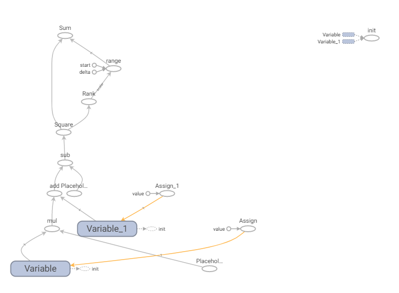
下面打代码中,实现了一个简单的线性模型,并绘制了其计算图,如下所示:
import tensorflow as tf
# import tensorflow.compat.v1 as tf

w = tf.Variable([0.3], dtype=tf.float32)
b = tf.Variable([-0.3], dtype=tf.float32)
x = tf.placeholder(dtype=tf.float32)
y = tf.placeholder(dtype=tf.float32)
linear_model = w*x+b
square_deltas = tf.square(linear_model-y)
loss = tf.reduce_sum(square_deltas)

init = tf.global_variables_initializer()
with tf.Session() as sess:
    sess.run(init)  # 初始权重值
    print("初始loss:", sess.run(loss, feed_dict={x: [1,  2,  3,  4], y: [0,  -1,  -2,  -3]}))

    fix_w = tf.assign(w, [-1])
    fix_b = tf.assign(b, [1])
    sess.run([fix_w, fix_b])  # 更新权重值
    print("更新权重后loss: ", sess.run(loss, feed_dict={x: [1,  2,  3,  4], y: [0,  -1,  -2,  -3]}))

    tf.summary.FileWriter("./logs", sess.graph)  # 在tensorboard中绘制计算图
对应的计算图:
5. tf.train 相关API
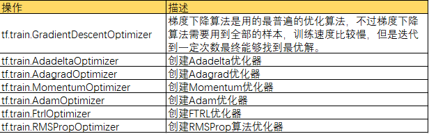
了解上述知识点后,可以开始搭建简单的网络,并进行训练。tf.train提供了关于优化器相关的函数,可以实现梯度梯度下降和参数更新。
常用优化器:
常用损失函数:
- tf.nn
在tensorflow原生库中,只有最常见的几种loss函数。
上面是softmax交叉熵loss,参数为网络最后一层的输出和onehot形式的标签。切记输入一定不要经过softmax,因为在函数中内置了softmax操作,如果再做就是重复使用了。在计算loss的时候,输出Tensor要加上tf.reduce_mean(Tensor)或者tf.reduce_sum(Tensor),作为tensorflow优化器(optimizer)的输入。
这个函数和上面的区别就是labels参数应该是没有经过onehot的标签,其余的都是一样的。另外加了sparse的loss还有一个特性就是标签可以出现-1,如果标签是-1代表这个数据不再进行梯度回传。
sigmoid交叉熵loss,与softmax不同的是,该函数首先进行sigmoid操作之后计算交叉熵的损失函数,其余的特性与 一致。
这个loss与众不同的地方就是加入了一个权重的系数,其余的地方与 这个损失函数是一致的,加入的pos_weight函数可以适当的增大或者缩小正样本的loss,可以一定程度上解决正负样本数量差距过大的问题。
- tf.keras
中是全部的loss函数库,但是也只是非常普通有限的函数。
下面代码中采用tensorflow实现了一个多层感知机,并对minist数据集进行分类:(minist数据集:手写数字灰度图片)


import tensorflow as tf
from keras.datasets import mnist

(x_train, y_train), (x_test, y_test) = mnist.load_data()
# print(x_train.shape, y_train.shape, x_test.shape)


nClass = tf.placeholder(tf.int32)
x = tf.placeholder(tf.float32, shape=[None, 784])
y = tf.placeholder(tf.int32, shape=[None])
y_hot = tf.one_hot(indices=y, depth=nClass, on_value=1.0, off_value=0.0, axis=-1)

# 网络层
w1 = tf.Variable(initial_value=tf.random_normal(shape=[784, 100], stddev=0.1), name="weight1")
b1 = tf.Variable(initial_value=tf.constant(0.1, shape=(1, 100)), name="bias1")
h1 = tf.nn.relu(tf.matmul(x, w1)+b1)

w2 = tf.Variable(initial_value=tf.random_normal(shape=[100, 20], stddev=0.1), name="weight2")
b2 = tf.Variable(initial_value=tf.constant(0.1, shape=(1, 20)), name="bias2")
h2 = tf.nn.relu(tf.matmul(h1, w2)+b2)

w3 = tf.Variable(initial_value=tf.random_normal(shape=[20, 10], stddev=0.1), name="weight2")
b3 = tf.Variable(initial_value=tf.constant(0.1, shape=(1, 10)), name="bias2")
h3 = tf.matmul(h2, w3)+b3

cross_entropy = tf.reduce_mean(tf.nn.softmax_cross_entropy_with_logits(labels=y_hot, logits=h3))
# train_step = tf.train.GradientDescentOptimizer(0.1).minimize(cross_entropy)   # 梯度下降法,学习率为0.01
train_step = tf.train.AdamOptimizer(0.0001).minimize(cross_entropy)   # 梯度下降法,学习率为0.01


# 测试
prediction = tf.equal(tf.argmax(h3, axis=1), tf.argmax(y_hot, axis=1))
accuracy = tf.reduce_mean(tf.cast(prediction, dtype=tf.float32))

with tf.Session() as sess:
    epochs = 300
    batch_size = 8
    n = x_train.shape[0]
    # n = 10000
    sess.run(tf.global_variables_initializer())

    for epoch in range(epochs):
        epoch_loss = 0.0
        iter_count = 0
        for i in range(0, n, batch_size):
            j = min(i + batch_size, n)
            batch_data = x_train[i:j, :, :].reshape(-1, 28 * 28)
            batch_label = y_train[i:j]
            _, loss = sess.run([train_step, cross_entropy], feed_dict={x: batch_data, y: batch_label, nClass: 10})
            # if epoch % 40 == 0:
            #     train_accuracy = accuracy.eval(feed_dict={
            #         x: batch_data, y: batch_label, nClass: 10})
            #     print('step %d, training accuracy %g' % (i, train_accuracy))
            epoch_loss += loss
            iter_count += 1

        print("[Epoch {}/{}], train loss: {}".format(epoch, epochs, epoch_loss/iter_count))


    # 测试:
    acc = 0
    iter_count = 0
    n = x_test.shape[0]
    for i in range(0, n, batch_size):
        j = min(i + batch_size, n)
        batch_data = x_test[i:j, :, :].reshape(-1, 28 * 28)
        batch_label = y_test[i:j]
        acc += sess.run(accuracy, feed_dict={x:batch_data, y:batch_label, nClass:10})
        iter_count += 1

    print('Test accuracy {:.4f}%'.format(100*acc/iter_count))    # Test accuracy 92.3077%
6. 正则化损失
一般为了防止过拟合,会采用L2正则化,tensorflow中的L2正则化使用起来有点特别。
下面代码中实现了cifar10数据集的分类,并采用了tf.nn.l2_loss来实现网络参数的L2正则化,限制网络规模,从而达到抑制过拟合的目的:
import tensorflow as tf
# import tensorflow.compat.v1 as tf
import Cifar10_data
import time
import math
import numpy as np

# 创建一个variable_with_weight_loss()函数,该函数的作用是:
#   1.使用参数w1控制L2 loss的大小
#   2.使用函数tf.nn.l2_loss()计算权重L2 loss
#   3.使用函数tf.multiply()计算权重L2 loss与w1的乘积,并赋值给weights_loss
#   4.使用函数tf.add_to_collection()将最终的结果放在名为losses的集合里面,方便后面计算神经网络的总体loss,
def variable_with_weight_loss(shape, stddev, w):
    var = tf.Variable(tf.truncated_normal(shape=shape, stddev=0.1))   # 截断的正态分布,超过两倍标准偏差的被舍弃掉
    if w is not None:
        weight_loss = tf.multiply(tf.nn.l2_loss(var), w, name="weight_loss")
        tf.add_to_collection("losses", weight_loss)
    return var


def conv2d(x, w, strides):
    return tf.nn.conv2d(x, w, strides, padding='SAME')
    #图片X:shape(batch,h,w,channel); 卷积核w:(h,w,in_channel, out_channel); strides:[1, stride, stride, 1];
    # padding: 'SAME'考虑边界,填充0,'VALID'不填充边界


# 1. 参数设置
batch_size = 32
cifar_data_dir = r"./cifar_data/cifar-10-batches-bin"  # 二进制文件格式存放
num_examples_for_eval = 10000   # 10000张测试图片
num_examples_for_train = 50000  # 50000 张训练图片;   (一个epoch训练:50000/8 个batch)
max_steps =  int(math.ceil(num_examples_for_train)/batch_size)*300   # 训练300个epoch


# 2. 数据加载
# from keras.datasets import cifar10
# (x_train, y_train), (x_test, y_test) = cifar10.load_data()
images_train, labels_train = Cifar10_data.inputs(data_dir=cifar_data_dir, batch_size=batch_size, distorted=True)
images_test, labels_test = Cifar10_data.inputs(data_dir=cifar_data_dir, batch_size=batch_size, distorted=None)
print(images_train.shape, labels_train.shape, images_test.shape, labels_test.shape)


# 3. 网络搭建
x = tf.placeholder(dtype=tf.float32, shape=[batch_size, 24, 24, 3])  # cifar10: 32*32*3, 前处理crop到24*24*3
y_ = tf.placeholder(dtype=tf.int32, shape=[batch_size])

# 卷积层1
w_conv1 = variable_with_weight_loss(shape=[5, 5, 3, 64], stddev=5e-2, w=0)  # 卷积核输入channel是3,输出channel是64
b_conv1 = tf.Variable(tf.constant(0.0, shape=[64]))  # 初始化为0
h_conv1 = tf.nn.relu(conv2d(x, w_conv1, strides=[1, 1, 1, 1])+b_conv1)
h_pool1 = tf.nn.max_pool(h_conv1, ksize=[1, 3, 3, 1], strides=[1, 2, 2, 1], padding='SAME')

# 卷积层2
w_conv2 = variable_with_weight_loss([5,5,64,64], stddev=5e-2, w=0)
b_conv2 = tf.Variable(tf.constant(0.1, shape=[64]))
h_conv2 = tf.nn.relu(conv2d(h_pool1, w_conv2, strides=[1, 1, 1, 1])+b_conv2)
h_pool2 = tf.nn.max_pool(h_conv1, ksize=[1, 3, 3, 1], strides=[1, 2, 2, 1], padding='SAME')

# reshape
x_flat = tf.reshape(h_pool2, shape=[batch_size, -1])  # h_pool2:shape(7,7,64),需要reshape,方便全连接
dim = x_flat.get_shape()[1].value

# 全连接层1
w_fc1 = variable_with_weight_loss([dim, 384], stddev=0.04, w=0.004)
b_fc1 = tf.Variable(tf.constant(0.1, shape=[384]))
h_fc1 = tf.nn.relu(tf.matmul(x_flat, w_fc1) + b_fc1)

# 全连接层2
w_fc2 = variable_with_weight_loss([384, 192], stddev=0.04, w=0.004)
b_fc2 = tf.Variable(tf.constant(0.1, shape=[192]))
h_fc2 = tf.nn.relu(tf.matmul(h_fc1, w_fc2) + b_fc2)

# dropout
keep_prob = tf.placeholder(tf.float32)  # train是设置丢弃概率;eval时可以设置为1
h_fc2_drop = tf.nn.dropout(h_fc2, keep_prob)

# 全连接层3,预测输出
w_fc3 = variable_with_weight_loss([192, 10], stddev=1 / 192.0, w=0.0)
b_fc3 = tf.Variable(tf.constant(0.1, shape=[10]))
y_output = tf.add(tf.matmul(h_fc2_drop, w_fc3), b_fc3)

# 损失函数
#loss = tf.reduce_mean(tf.nn.softmax_cross_entropy_logits(labels=y_, logits=y_output))
cross_entropy=tf.nn.sparse_softmax_cross_entropy_with_logits(labels=tf.cast(y_,tf.int64), logits=y_output)
weights_with_l2_loss = tf.add_n(tf.get_collection("losses"))
loss = tf.reduce_mean(cross_entropy) + weights_with_l2_loss

# 训练优化器
train_step = tf.train.AdamOptimizer(0.001).minimize(loss)


# 测试
top_k_op = tf.nn.in_top_k(y_output, y_, 1)  # 计算输出结果中top k的准确率,函数默认的k值是1,即top 1的准确率,也就是输出分类准确率最高时的数值
# correct_prediction = tf.equal(tf.argmax(y_output, 1), tf.argmax(y_, 1))
# accuracy = tf.reduce_mean(tf.cast(correct_prediction, dtype=tf.float32))  # cast数据转换

with tf.Session() as sess:
    sess.run(tf.global_variables_initializer())  # 初始化定义的变量
    # 启动线程操作,这是因为之前数据增强的时候使用train.shuffle_batch()函数的时候通过参数num_threads()配置了16个线程用于组织batch的操作
    tf.train.start_queue_runners()

    for step in range(max_steps):
            t1 = time.time()
            image_batch, label_batch = sess.run([images_train, labels_train])   #返回一个batch的数据
            # print(step, image_batch.shape, label_batch)
            loss_value, _ = sess.run([loss, train_step], feed_dict={x: image_batch, y_: label_batch, keep_prob: 0.5})
            duration = time.time() - t1
            if step % 100 == 0:
                # train_accuracy = accuracy.eval(feed_dict={
                #     x: image_batch, y_: label_batch, keep_prob: 1.0})
                print("[Step {}/{}] loss={:.4f}, {:.1f} images/sec, {} sec/batch".format(
                    step, max_steps, loss_value, batch_size/duration, duration))

    # 测试阶段
    num_batch = int(math.ceil(num_examples_for_eval/batch_size))  # 有多少个batch
    true_count = 0
    total_sample_count=num_batch * batch_size   # 若最后一个batch,图片不够一个batch_size时,注意是如何处理的?
    for i in range(num_batch):
        image_batch, label_batch = sess.run([images_test, labels_test])
        predictions = sess.run([top_k_op], feed_dict={x: image_batch, y_: label_batch, keep_prob: 1})
        true_count += np.sum(predictions)
    print("Test accuracy: {:.4f}%".format(100*true_count/total_sample_count))
# 该文件负责读取Cifar-10数据并对其进行数据增强预处理
import os
import tensorflow as tf

num_classes = 10

# 设定用于训练和评估的样本总数
num_examples_pre_epoch_for_train = 50000
num_examples_pre_epoch_for_eval = 10000


# 定义一个空类,用于返回读取的Cifar-10的数据
class CIFAR10Record(object):
    pass


# 定义一个读取Cifar-10的函数read_cifar10(),这个函数的目的就是读取目标文件里面的内容
def read_cifar10(file_queue):
    result = CIFAR10Record()

    label_bytes = 1  # 如果是Cifar-100数据集,则此处为2
    result.height = 32
    result.width = 32
    result.depth = 3  # 因为是RGB三通道,所以深度是3

    image_bytes = result.height * result.width * result.depth  # 图片样本总元素数量
    record_bytes = label_bytes + image_bytes  # 因为每一个样本包含图片和标签,所以最终的元素数量还需要图片样本数量加上一个标签值

    reader = tf.FixedLengthRecordReader(
        record_bytes=record_bytes)  # 使用tf.FixedLengthRecordReader()创建一个文件读取类。该类的目的就是读取文件
    result.key, value = reader.read(file_queue)  # 使用该类的read()函数从文件队列里面读取文件

    record_bytes = tf.decode_raw(value, tf.uint8)  # 读取到文件以后,将读取到的文件内容从字符串形式解析为图像对应的像素数组

    # 因为该数组第一个元素是标签,所以我们使用strided_slice()函数将标签提取出来,并且使用tf.cast()函数将这一个标签转换成int32的数值形式
    result.label = tf.cast(tf.strided_slice(record_bytes, [0], [label_bytes]), tf.int32)

    # 剩下的元素再分割出来,这些就是图片数据,因为这些数据在数据集里面存储的形式是depth * height * width,我们要把这种格式转换成[depth,height,width]
    # 这一步是将一维数据转换成3维数据
    depth_major = tf.reshape(tf.strided_slice(record_bytes, [label_bytes], [label_bytes + image_bytes]),
                             [result.depth, result.height, result.width])

    # 我们要将之前分割好的图片数据使用tf.transpose()函数转换成为高度信息、宽度信息、深度信息这样的顺序
    # 这一步是转换数据排布方式,变为(h,w,c)
    result.uint8image = tf.transpose(depth_major, [1, 2, 0])

    return result  # 返回值是已经把目标文件里面的信息都读取出来


def inputs(data_dir, batch_size, distorted):  # 这个函数就对数据进行预处理---对图像数据是否进行增强进行判断,并作出相应的操作
    filenames = [os.path.join(data_dir, "data_batch_%d.bin" % i) for i in range(1, 6)]  # 拼接地址

    file_queue = tf.train.string_input_producer(filenames)  # 根据已经有的文件地址创建一个文件队列
    read_input = read_cifar10(file_queue)  # 根据已经有的文件队列使用已经定义好的文件读取函数read_cifar10()读取队列中的文件

    reshaped_image = tf.cast(read_input.uint8image, tf.float32)  # 将已经转换好的图片数据再次转换为float32的形式

    num_examples_per_epoch = num_examples_pre_epoch_for_train

    if distorted != None:  # 如果预处理函数中的distorted参数不为空值,就代表要进行图片增强处理
        cropped_image = tf.random_crop(reshaped_image, [24, 24, 3])  # 首先将预处理好的图片进行剪切,使用tf.random_crop()函数

        flipped_image = tf.image.random_flip_left_right(
            cropped_image)  # 将剪切好的图片进行左右翻转,使用tf.image.random_flip_left_right()函数

        adjusted_brightness = tf.image.random_brightness(flipped_image,
                                                         max_delta=0.8)  # 将左右翻转好的图片进行随机亮度调整,使用tf.image.random_brightness()函数

        adjusted_contrast = tf.image.random_contrast(adjusted_brightness, lower=0.2,
                                                     upper=1.8)  # 将亮度调整好的图片进行随机对比度调整,使用tf.image.random_contrast()函数

        float_image = tf.image.per_image_standardization(
            adjusted_contrast)  # 进行标准化图片操作,tf.image.per_image_standardization()函数是对每一个像素减去平均值并除以像素方差

        float_image.set_shape([24, 24, 3])  # 设置图片数据及标签的形状
        read_input.label.set_shape([1])

        min_queue_examples = int(num_examples_pre_epoch_for_eval * 0.4)
        print("Filling queue with %d CIFAR images before starting to train.    This will take a few minutes."
              % min_queue_examples)

        images_train, labels_train = tf.train.shuffle_batch([float_image, read_input.label], batch_size=batch_size,
                                                            num_threads=4,
                                                            capacity=min_queue_examples + 3 * batch_size,
                                                            min_after_dequeue=min_queue_examples,
                                                            )
        # 使用tf.train.shuffle_batch()函数随机产生一个batch的image和label

        return images_train, tf.reshape(labels_train, [batch_size])

    else:  # 不对图像数据进行数据增强处理
        resized_image = tf.image.resize_image_with_crop_or_pad(reshaped_image, 24,
                                                               24)  # 在这种情况下,使用函数tf.image.resize_image_with_crop_or_pad()对图片数据进行剪切

        float_image = tf.image.per_image_standardization(resized_image)  # 剪切完成以后,直接进行图片标准化操作

        float_image.set_shape([24, 24, 3])
        read_input.label.set_shape([1])

        min_queue_examples = int(num_examples_per_epoch * 0.4)

        images_test, labels_test = tf.train.batch([float_image, read_input.label],
                                                  batch_size=batch_size, num_threads=4,
                                                  capacity=min_queue_examples + 3 * batch_size)
        # 这里使用batch()函数代替tf.train.shuffle_batch()函数
        return images_test, tf.reshape(labels_test, [batch_size])
7. 数据集加载
tensorflow中tf.data.Dataset 和tf.train.slice_input_producer都提供了数据集的批量加载方式。
1. tf.train.slice_input_producer
如果我们的数据保存在txt文件中,txt文件格式如下, 即每一行是图片路径和label
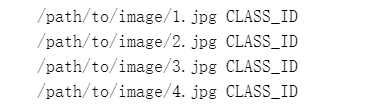
则加载图片的dataloder,数据加载代码如下:
def read_images(dataset_path, batch_size, transform=False):
    # 1. slice_input_producer构建一个任务队列
    imagepaths, labels = list(), list()

    with open(dataset_path) as f:
        data = f.read().splitlines()
    for d in data:
        imagepaths.append(d.split(' ')[0])
        labels.append(int(d.split(' ')[1]))

    # Convert to Tensor
    imagepaths = tf.convert_to_tensor(imagepaths, dtype=tf.string)
    labels = tf.convert_to_tensor(labels, dtype=tf.int32)
    # Build a TF Queue, shuffle data
    image, label = tf.train.slice_input_producer([imagepaths, labels],
                                                 shuffle=True)
    # 2. 对图片和lable可以进行预处理
    # Read images from disk
    image = tf.read_file(image)
    image = tf.image.decode_jpeg(image, channels=CHANNELS)

    if transform:  # 是否要进行图片增强处理
        cropped_image = tf.random_crop(image, [24, 24, 3])  # 首先将预处理好的图片进行剪切,使用tf.random_crop()函数

        flipped_image = tf.image.random_flip_left_right(
            cropped_image)  # 将剪切好的图片进行左右翻转,使用tf.image.random_flip_left_right()函数

        adjusted_brightness = tf.image.random_brightness(flipped_image,
                                                         max_delta=0.8)  # 将左右翻转好的图片进行随机亮度调整,使用tf.image.random_brightness()函数

        adjusted_contrast = tf.image.random_contrast(adjusted_brightness, lower=0.2,
                                                     upper=1.8)  # 将亮度调整好的图片进行随机对比度调整,使用tf.image.random_contrast()函数

        float_image = tf.image.per_image_standardization(
            adjusted_contrast)  # 进行标准化图片操作,tf.image.per_image_standardization()函数是对每一个像素减去平均值并除以像素方差

        image = float_image
        image.set_shape([24, 24, 3])  # 设置图片数据及标签的形状
        label.set_shape([1])

    # Resize images to a common size
    image = tf.image.resize_images(image, [IMG_HEIGHT, IMG_WIDTH])

    # Normalize
    image = image * 1.0 / 127.5 - 1.0

    # 3. 创建一个batch生成器
    # Create batches
    X, Y = tf.train.batch([image, label], batch_size=batch_size,
                          capacity=batch_size * 8,   # 任务队列的大小
                          num_threads=4)  # 四个线程进行数据加载

    # X,Y = tf.train.shuffle_batch([image, label], batch_size=batch_size,
    #                                                     num_threads=4,
    #                                                     capacity=min_queue_examples + 3 * batch_size,
    #                                                     min_after_dequeue=min_queue_examples,
    #                                                     )

    return X, Y
图片加载和整个训练代码如下,使用tf.train.slice_input_producer()产生队列后,注意在训练时得通过tf.train.start_queue_runners()开始队列
import tensorflow as tf
import os

# Dataset Parameters - CHANGE HERE
MODE = 'folder' # or 'file', if you choose a plain text file (see above).
DATASET_PATH = '/path/to/dataset/' # the dataset file or root folder path.

# Image Parameters
N_CLASSES = 2 # CHANGE HERE, total number of classes
IMG_HEIGHT = 64 # CHANGE HERE, the image height to be resized to
IMG_WIDTH = 64 # CHANGE HERE, the image width to be resized to
CHANNELS = 3 # The 3 color channels, change to 1 if grayscale


def read_images(dataset_path, batch_size, transform=False):
    # 1. slice_input_producer构建一个任务队列
    imagepaths, labels = list(), list()

    with open(dataset_path) as f:
        data = f.read().splitlines()
    for d in data:
        imagepaths.append(d.split(' ')[0])
        labels.append(int(d.split(' ')[1]))

    # Convert to Tensor
    imagepaths = tf.convert_to_tensor(imagepaths, dtype=tf.string)
    labels = tf.convert_to_tensor(labels, dtype=tf.int32)
    # Build a TF Queue, shuffle data
    image, label = tf.train.slice_input_producer([imagepaths, labels],
                                                 shuffle=True)
    # 2. 对图片和lable可以进行预处理
    # Read images from disk
    image = tf.read_file(image)
    image = tf.image.decode_jpeg(image, channels=CHANNELS)

    if transform:  # 是否要进行图片增强处理
        cropped_image = tf.random_crop(image, [24, 24, 3])  # 首先将预处理好的图片进行剪切,使用tf.random_crop()函数

        flipped_image = tf.image.random_flip_left_right(
            cropped_image)  # 将剪切好的图片进行左右翻转,使用tf.image.random_flip_left_right()函数

        adjusted_brightness = tf.image.random_brightness(flipped_image,
                                                         max_delta=0.8)  # 将左右翻转好的图片进行随机亮度调整,使用tf.image.random_brightness()函数

        adjusted_contrast = tf.image.random_contrast(adjusted_brightness, lower=0.2,
                                                     upper=1.8)  # 将亮度调整好的图片进行随机对比度调整,使用tf.image.random_contrast()函数

        float_image = tf.image.per_image_standardization(
            adjusted_contrast)  # 进行标准化图片操作,tf.image.per_image_standardization()函数是对每一个像素减去平均值并除以像素方差

        image = float_image
        image.set_shape([24, 24, 3])  # 设置图片数据及标签的形状
        label.set_shape([1])

    # Resize images to a common size
    image = tf.image.resize_images(image, [IMG_HEIGHT, IMG_WIDTH])

    # Normalize
    image = image * 1.0 / 127.5 - 1.0

    # 3. 创建一个batch生成器
    # Create batches
    X, Y = tf.train.batch([image, label], batch_size=batch_size,
                          capacity=batch_size * 8,   # 任务队列的大小
                          num_threads=4)  # 四个线程进行数据加载

    # X,Y = tf.train.shuffle_batch([image, label], batch_size=batch_size,
    #                                                     num_threads=4,
    #                                                     capacity=min_queue_examples + 3 * batch_size,
    #                                                     min_after_dequeue=min_queue_examples,
    #                                                     )

    return X, Y


# Parameters
learning_rate = 0.001
num_steps = 10000
batch_size = 128
display_step = 100

# Network Parameters
dropout = 0.75 # Dropout, probability to keep units

# Build the data input
X, Y = read_images(DATASET_PATH, MODE, batch_size)


# 模型搭建

# Create model
def conv_net(x, n_classes, dropout, reuse, is_training):
    # Define a scope for reusing the variables
    with tf.variable_scope('ConvNet', reuse=reuse):

        # Convolution Layer with 32 filters and a kernel size of 5
        conv1 = tf.layers.conv2d(x, 32, 5, activation=tf.nn.relu)
        # Max Pooling (down-sampling) with strides of 2 and kernel size of 2
        conv1 = tf.layers.max_pooling2d(conv1, 2, 2)

        # Convolution Layer with 32 filters and a kernel size of 5
        conv2 = tf.layers.conv2d(conv1, 64, 3, activation=tf.nn.relu)
        # Max Pooling (down-sampling) with strides of 2 and kernel size of 2
        conv2 = tf.layers.max_pooling2d(conv2, 2, 2)

        # Flatten the data to a 1-D vector for the fully connected layer
        fc1 = tf.contrib.layers.flatten(conv2)

        # Fully connected layer (in contrib folder for now)
        fc1 = tf.layers.dense(fc1, 1024)
        # Apply Dropout (if is_training is False, dropout is not applied)
        fc1 = tf.layers.dropout(fc1, rate=dropout, training=is_training)

        # Output layer, class prediction
        out = tf.layers.dense(fc1, n_classes)
        # Because 'softmax_cross_entropy_with_logits' already apply softmax,
        # we only apply softmax to testing network
        out = tf.nn.softmax(out) if not is_training else out

    return out


# 训练代码

# Because Dropout have different behavior at training and prediction time, we
# need to create 2 distinct computation graphs that share the same weights.

# Create a graph for training
logits_train = conv_net(X, N_CLASSES, dropout, reuse=False, is_training=True)
# Create another graph for testing that reuse the same weights
logits_test = conv_net(X, N_CLASSES, dropout, reuse=True, is_training=False)

# Define loss and optimizer (with train logits, for dropout to take effect)
loss_op = tf.reduce_mean(tf.nn.sparse_softmax_cross_entropy_with_logits(
    logits=logits_train, labels=Y))
optimizer = tf.train.AdamOptimizer(learning_rate=learning_rate)
train_op = optimizer.minimize(loss_op)

# Evaluate model (with test logits, for dropout to be disabled)
correct_pred = tf.equal(tf.argmax(logits_test, 1), tf.cast(Y, tf.int64))
accuracy = tf.reduce_mean(tf.cast(correct_pred, tf.float32))

# Initialize the variables (i.e. assign their default value)
init = tf.global_variables_initializer()

# Saver object
saver = tf.train.Saver()

# Start training
with tf.Session() as sess:

    # Run the initializer
    sess.run(init)

    # Start the data queue
    tf.train.start_queue_runners()

    # Training cycle
    for step in range(1, num_steps+1):

        if step % display_step == 0:
            # Run optimization and calculate batch loss and accuracy
            _, loss, acc = sess.run([train_op, loss_op, accuracy])
            print("Step " + str(step) + ", Minibatch Loss= " + \
                  "{:.4f}".format(loss) + ", Training Accuracy= " + \
                  "{:.3f}".format(acc))
        else:
            # Only run the optimization op (backprop)
            sess.run(train_op)

    print("Optimization Finished!")

    # Save your model
    saver.save(sess, 'my_tf_model')
2. tf.data.Dataset:
如果我们的数据和标签都是np.array类似,可以采用如下的加载方式:
import numpy as np
import tensorflow as tf

evens = np.arange(0, 100, step=2, dtype=np.int32)
evens_label = np.zeros(50, dtype=np.int32)
odds = np.arange(1, 100, step=2, dtype=np.int32)
odds_label = np.ones(50, dtype=np.int32)
# Concatenate arrays
features = np.concatenate([evens, odds])      # 数据:shape(100, )
labels = np.concatenate([evens_label, odds_label]) # 标签:shape(100,)
# print(features.shape, labels.shape)


def dataloader(features, labels):
    # Slice the numpy arrays (each row becoming a record).
    data = tf.data.Dataset.from_tensor_slices((features, labels))
    # Refill data indefinitely.
    data = data.repeat()
    # Shuffle data.
    data = data.shuffle(buffer_size=100)
    # Batch data (aggregate records together).
    data = data.batch(batch_size=4)
    # Prefetch batch (pre-load batch for faster consumption).
    data = data.prefetch(buffer_size=1)

    # Create an iterator over the dataset.
    iterator = data.make_initializable_iterator()

    return iterator

    # # Initialize the iterator.
    # sess.run(iterator.initializer)
    #
    # # Get next data batch.
    # d = iterator.get_next()
    #
    # return d

with tf.Session() as sess:

    iterator = dataloader(features, labels)
    sess.run(iterator.initializer)   # Initialize the iterator.
    dataloader = iterator.get_next()

    # Display data.
    for i in range(5):
        x, y = sess.run(dataloader)
        print(x, y)
如果我们加载如下的图片数据, 下面有一个加载 Oxford Flowers dataset的示例代码:
d = requests.get("http://www.robots.ox.ac.uk/~vgg/data/flowers/17/17flowers.tgz")
with open("17flowers.tgz", "wb") as f:
    f.write(d.content)
# Extract archive.
with tarfile.open("17flowers.tgz") as t:
    t.extractall()

# Create a file to list all images path and their corresponding label.
with open('jpg/dataset.csv', 'w') as f:
    c = 0
    for i in range(1360):
        f.write("jpg/image_%04i.jpg,%i\n" % (i+1, c))
        if (i+1) % 80 == 0:
            c += 1

with tf.Graph().as_default():

    # Load Images.
    with open("jpg/dataset.csv") as f:
        dataset_file = f.read().splitlines()

    # Create TF session.
    sess = tf.Session()

    # Load the whole dataset file, and slice each line.
    data = tf.data.Dataset.from_tensor_slices(dataset_file)
    # Refill data indefinitely.
    data = data.repeat()
    # Shuffle data.
    data = data.shuffle(buffer_size=1000)

    # Load and pre-process images.
    def load_image(path):
        # Read image from path.
        image = tf.io.read_file(path)
        # Decode the jpeg image to array [0, 255].
        image = tf.image.decode_jpeg(image)
        # Resize images to a common size of 256x256.
        image = tf.image.resize(image, [256, 256])
        # Rescale values to [-1, 1].
        image = 1. - image / 127.5
        return image
    # Decode each line from the dataset file.
    def parse_records(line):
        # File is in csv format: "image_path,label_id".
        # TensorFlow requires a default value, but it will never be used.
        image_path, image_label = tf.io.decode_csv(line, ["", 0])
        # Apply the function to load images.
        image = load_image(image_path)
        return image, image_label
    # Use 'map' to apply the above functions in parallel.
    data = data.map(parse_records, num_parallel_calls=4)

    # Batch data (aggregate images-array together).
    data = data.batch(batch_size=2)
    # Prefetch batch (pre-load batch for faster consumption).
    data = data.prefetch(buffer_size=1)

    # Create an iterator over the dataset.
    iterator = data.make_initializable_iterator()
    # Initialize the iterator.
    sess.run(iterator.initializer)

    # Get next data batch.
    d = iterator.get_next()

for i in range(1):
    batch_x, batch_y = sess.run(d)
    print(batch_x, batch_y)
8. 模型的保存和加载
Tensorflow有专门保存模型的tf.train.Saver(). 使用Saver保存模型的参数时,一定要将saver = tf.train.Saver定义在你保存的的参数定义之后,定义在saver之后的参数无法被保存。
如下面的代码,能将当前模型和其权值参数保存在tmp目录下
saver = tf.train.Saver()
saver.save(sess, "./tmp/model.ckpt")
上述代码会保存的文件如下:

其中后三个文件比较重要,依次存储的信息如下:
- .data文件:保存了当前参数值
- .index文件:保存了当前参数名
- .meta文件:保存了当前图结构
saver.save() 保存模型示例代码:
import numpy as np
import tensorflow as tf


class Network():
    x = tf.placeholder(shape=[1, None], dtype=tf.float32)
    y = tf.placeholder(shape=[1, None], dtype=tf.float32)

    inputW = tf.Variable(tf.random_normal([10, 1]))
    inputB = tf.Variable(tf.random_normal([10, 1]))

    hideW = tf.Variable(tf.random_normal([1, 10]))
    hideB = tf.Variable(tf.random_normal([1, 1]))

    h1 = tf.nn.sigmoid(tf.add(tf.matmul(inputW, x), inputB))
    output = tf.add(tf.matmul(hideW, h1), hideB)

    loss = tf.reduce_mean(tf.reduce_sum(tf.square(y - output)))

    opt = tf.train.AdamOptimizer(1)

    train_step = opt.minimize(loss)


if __name__ == '__main__':

    x_data = np.linspace(-1, 1, 100).reshape(1, 100)
    noise = np.random.normal(0, 0.05, x_data.shape)
    y_data = x_data ** 3 + 1 + noise

    net = Network()
    sess = tf.Session()
    init = tf.global_variables_initializer()

    sess.run(init)
    saver = tf.train.Saver()


    train_step = 200
    for step in range(train_step):
        print('第', step + 1, '次训练')
        sess.run(net.train_step, feed_dict={net.x: x_data, net.y: y_data})
        pre = sess.run(net.output, feed_dict={net.x: x_data})

    saver.save(sess, "./tmp/model.ckpt")
saver.load()载入上面保存的模型:
import tensorflow as tf
import numpy as np
import pylab as pl
from tensorflowtest import Network

sess = tf.Session()
saver = tf.train.Saver().restore(sess, "./tmp/model.ckpt")

net = Network()

x_data = np.linspace(-1,1,100).reshape(1,100)
pre = sess.run(net.output,feed_dict={net.x:x_data})


pl.plot(x_data.T,pre.T)
pl.grid()
pl.show()
参考: https://zhuanlan.zhihu.com/p/333791572
https://www.cnblogs.com/hellcat/p/6925757.html
https://zhuanlan.zhihu.com/p/31362241


 浙公网安备 33010602011771号