【R语言学习笔记】11. 线性回归中的交互效应(interaction)

 

1. 目的：构建线性回归模型并考虑自变量之间的交互效应。

 

2. 数据来源及背景

2.1 数据来源：数据为本人上课的案例数据，

2.2 数据背景：一公司想通过商品销售价格及是否提供打折来预测顾客购买商品的可能性。

library(car)
library(ggplot2)
library(jtools)

library(readxl)
luxury <- read_excel("Luxury.xlsx")
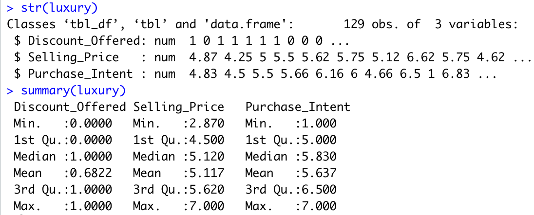
str(luxury)
summary(luxury)

 

 

 

3. 应用

3.1 数据初期探索

绘制变量间的散点图

# get the intuition of the data
ggplot(luxury, aes(x = Selling_Price, y = Purchase_Intent, col = as.factor(Discount_Offered))) + geom_point()

 

 

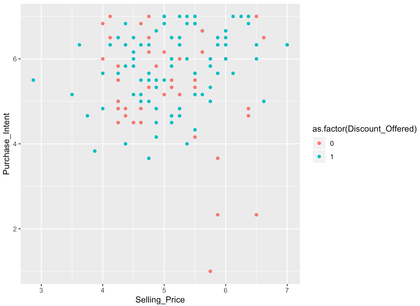
通过散点图，可以判断出：提供折扣时，商品价格越高，购买者越容易购买；不提供折扣时，商品价格越低，购买者越容易购买，故存在交互效应(interaction)。

 

3.2 构建模型

模型1：无交互作用的线性回归模型

step1：构建线性回归模型

# LM w/no interactions/moderators
l0 <- lm(Purchase_Intent ~ Selling_Price + Discount_Offered, data = luxury)
summary(l0)

 

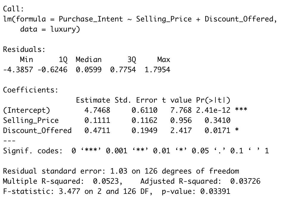
由模型结果可知，销售价格对于购买意向的回归并不显著。

 

step2：交叉检验及模型预测准确性：

# Create the splitting plan for 3-fold cross validation
set.seed(123)  # set the seed for reproducibility
library(vtreat)
splitPlan <- kWayCrossValidation(nrow(luxury), 3, NULL, NULL)

# get cross-val predictions for main-effects only model
luxury$lm.pred <- 0  # initialize the prediction vector
for(i in 1:3) {
  split <- splitPlan[[i]]
  lm <- lm(Purchase_Intent ~ Selling_Price + Discount_Offered, data = luxury[split$train, ])
  luxury$lm.pred[split$app] <- predict(l0, newdata = luxury[split$app, ])
}

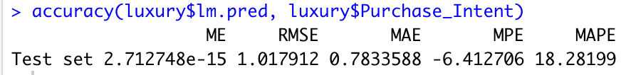
library(forecast)
accuracy(luxury$l0.pred, luxury$Purchase_Intent)

 

 

 

模型2：考虑交互作用的回归模型

step1：对数据做中心化处理

# mean-center predictors#
luxury$Mean_Center_Selling <- luxury$Selling_Price - mean(luxury$Selling_Price)
# alternative1
# luxury$Mean_Center_Selling <- c(scale(luxury$Selling_Price,center = TRUE,scale = FALSE))
# alternative2: preProcess(data, method = 'center')

 

step2：构建模型

#LM Interaction w/mean Centering#
l1 <- lm(Purchase_Intent ~ Discount_Offered * Mean_Center_Selling
       , data = luxury)
summary(l1)

 

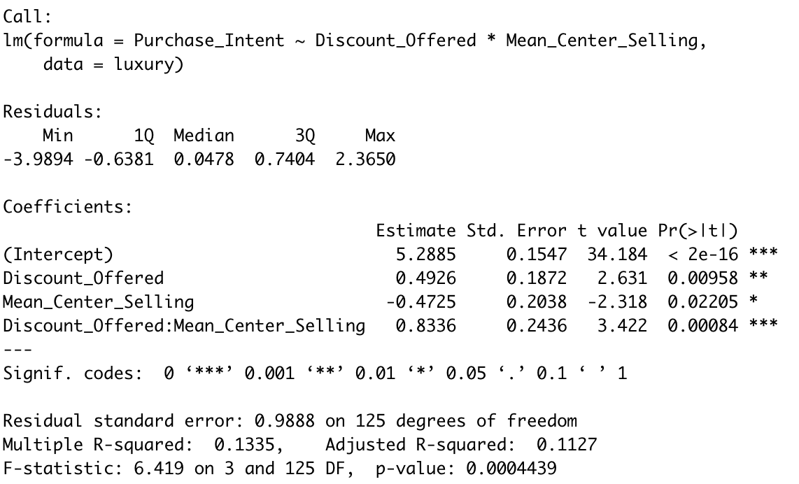
此时，全部自变量均与因变量显著相关，且R-squared显著提升。

 

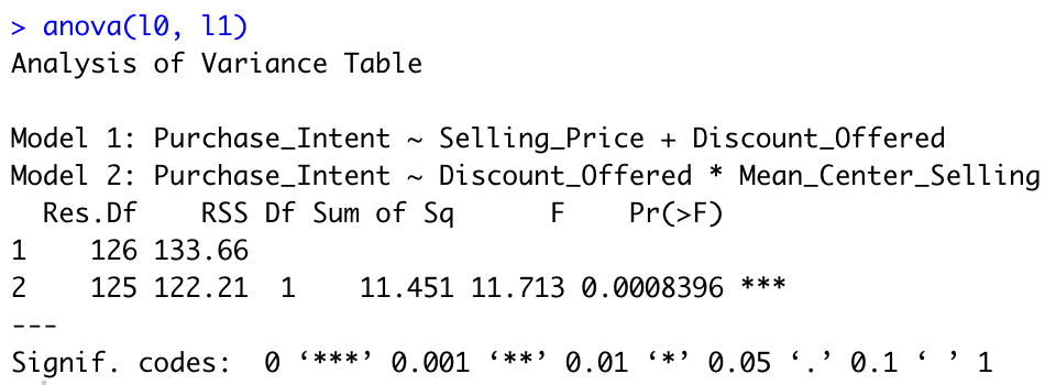
step3：F检验检测与模型1相比模型2是否显著改进

# F test
anova(l0, l1)

 

 

 

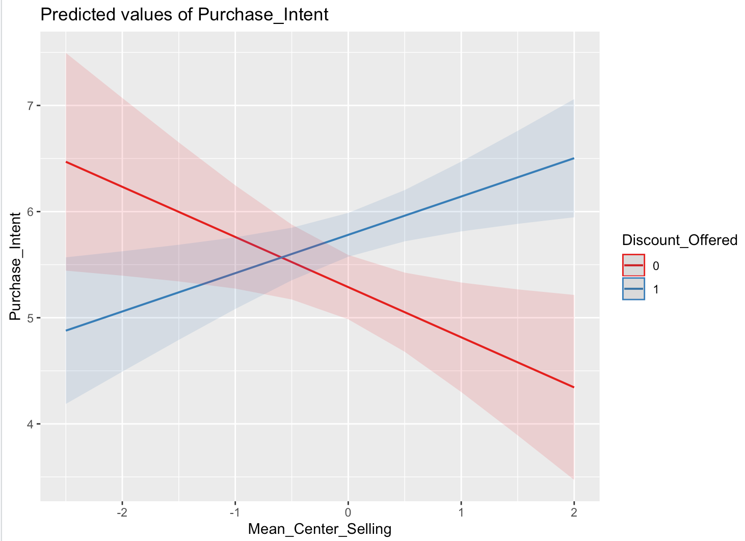
step4：绘制interaction plot

plot1

# interaction plot
library(sjPlot)
library(sjmisc)
plot_model(l1, type = "pred", terms = c('Mean_Center_Selling', 'Discount_Offered'))

 

 

 

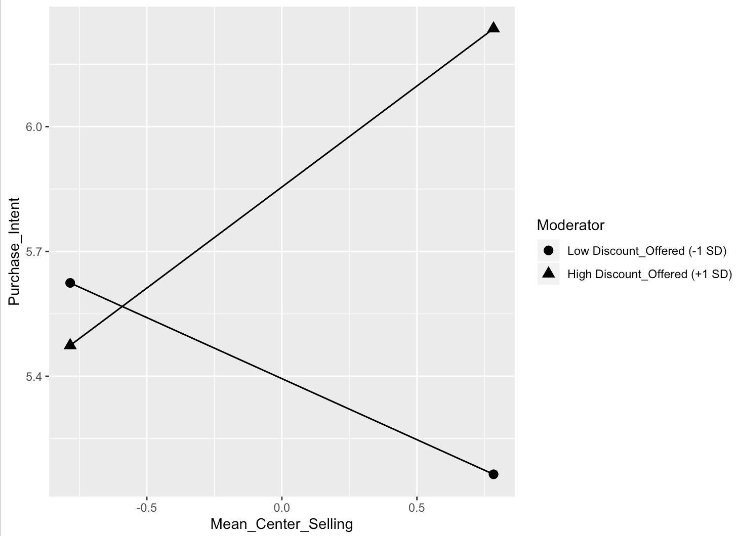
plot2

# alternative
library(pequod)

# Fit moderated linear regression with both residual centering and mean centering methods.
l2 <- lmres(Purchase_Intent ~ Mean_Center_Selling * Discount_Offered, data=luxury)

# Simple slopes analysis for Moderated regression
s_slopes <- simpleSlope(l2, pred = "Mean_Center_Selling", mod1 ="Discount_Offered")
# object: an object of class "lmres": a moderated regression function.
# pred: name of the predictor variable
# mod1: name of the first moderator variable
# mod2: name of the second moderator variable. Default "none" is used in order to analyzing two way interaction

# Simple slopes plot
PlotSlope(s_slopes)

 

 

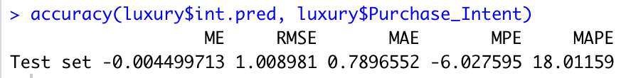
step5：交叉检验及模型预测准确性

# Get the cross-val predictions for the model with interactions
luxury$int.pred <- 0 # initialize the prediction vector
for(i in 1:3) {
  split <- splitPlan[[i]]
  int <- lm(Purchase_Intent ~ Mean_Center_Selling * Discount_Offered, data = luxury[split$train, ])
  luxury$int.pred[split$app] <- predict(int, newdata = luxury[split$app, ])
}

accuracy(luxury$int.pred, luxury$Purchase_Intent)

 

 

 

 

3.3 模型间准确性比较

# compare RMSE
library(tidyr)
library(dplyr)
luxury %>% 
  gather(key = modeltype, value = pred, lm.pred, int.pred) %>%
  mutate(residuals = Purchase_Intent - pred) %>%      
  group_by(modeltype) %>%
  summarize(rmse = sqrt(mean(residuals^2)))

 

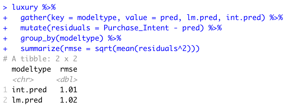
根据数据结果可知，模型2的RMSE比模型1的RMSE稍微小一点，但是R-squared显著提升。