【R语言学习笔记】9. 线性回归及其假设检验

 

1. 目的：构建线性回归模型并检验其假设是否成立。

 

2. 数据来源及背景

2.1 数据来源：数据为本人上课的案例数据，

2.2 数据背景：“玻璃制造公司”主要向新建筑承包商和汽车公司供应产品。该公司认为，他们的年销售额应与新建筑数量以及汽车生产高度相关，因此希望构建线性回归模型来预测其销售额。

 

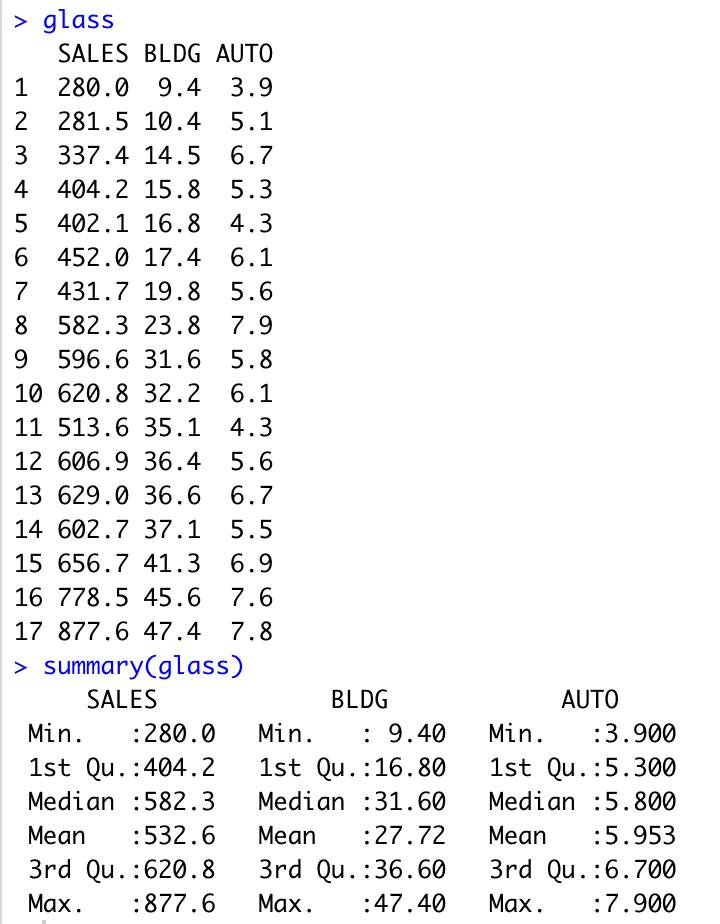
glass <- read.csv("glass_mult.csv",header=T)
glass
summary(glass)

　　

 

 

3. 应用

 

3.1 模型构建

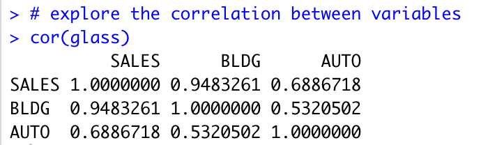
查看变量之间相关性，发现自变量BLDG与因变量SALES存在高达0.948的正相关性。

# explore the correlation between variables
cor(glass)

 

 

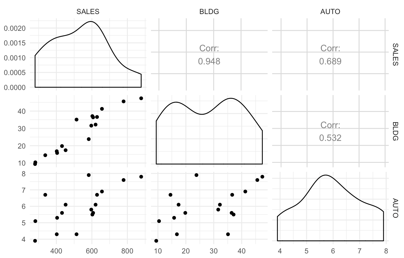
 绘制任意两个变量之间散点图来探索其相关关系。

# get all scatter plots between 2 variables
library(ggplot2)
library(GGally)
ggpairs(glass)
## alternative
## pairs( ~ SALES + BLDG + AUTO, data = glass)

 

 

 

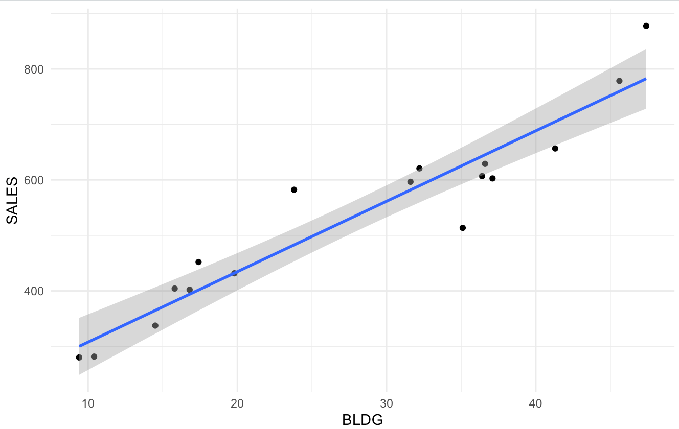
由于BLDG与SALES高度相关，故先构建二者之间的一元线性回归模型。

# build linear regression model 1
glass.lm1 <- lm(SALES ~ BLDG, data=glass)
summary(glass.lm1)
anova(glass.lm1)

 

根据模型结果，BLDG高度显著，且R-squared为0.8993，Adjusted R-squared为0.8926，说明该模型解释了将近90%的variance。

 

绘制BLDG与SALES的散点图，回归曲线，以及置信区间。

 

# plot the model as well as the real data
ggplot(glass, aes(x = BLDG, y = SALES)) + geom_point() + geom_smooth(method = 'lm') 
# could add se = 'F' to geom_smooth to remove standard error lines 

# alternative1
# ggplot(glass, aes(x = BLDG, y = SALES)) + geom_point() + 
# geom_abline(intercept = coef(glass.lm1)[1], slope = coef(glass.lm1)[2])

# alternative2
## plot(glass$BLDG, glass$SALES)
## abline(glass.lm1)

 

 

为了进一步理解一元线性回归模型，接下来手动构建一元线性回归模型并计算其参数(slope and intercept)。

# manually fit the simple linear regression model
library(dplyr)
glass %>%
  summarise(
    N = n(),
    r = cor(SALES, BLDG),
    mean_x = mean(BLDG),
    sd_x = sd(BLDG),
    mean_y = mean(SALES),
    sd_y = sd(SALES),
    slope = r * sd_y / sd_x,
    intercept = mean_y - slope * mean_x
  )

 

 

接下来，构建BLDG与AUTO的SALES模型。

# build linear regression model 2
glass.lm2 <- lm(SALES ~ BLDG+AUTO, data=glass)
summary(glass.lm2)
anova(glass.lm2)

 

根据模型结果，两个自变量均高度显著，且R-squred及Adjusted R-squred分别提高至0.9446和0.939。

 

 

探索模型二是否在模型一的基础上具有显著的提升。由于P-value小于0.05，我们可以认为模型二与模型一相比有显著提升。

# check model improvement
anova(glass.lm1, glass.lm2) # significant  p-value means significant improvement

 

  

基于已有数据，运用模型二对其进行预测，并绘制真实值与预测值的散点图来观察预测准确性。

# model prediction
glass$lm2.pred <- predict(glass.lm2)
# compare the model prediction and the real data points
ggplot(glass, aes(x = lm2.pred, y = SALES)) + geom_point() + geom_abline()

　　

 

 

 

3.2 检验模型是否符合线性回归的假设

假设1: 自变量之间是独立的 (independence)

该假设可以通过3.1中探索变量之间的相关性来验证。若自变量之间的相关性小于0.7，则可认为符合假设。

 

假设2：自变量与因变量之间为线性/可加性的关系 (linearity)

该假设可以通过绘制散点图来判断

 

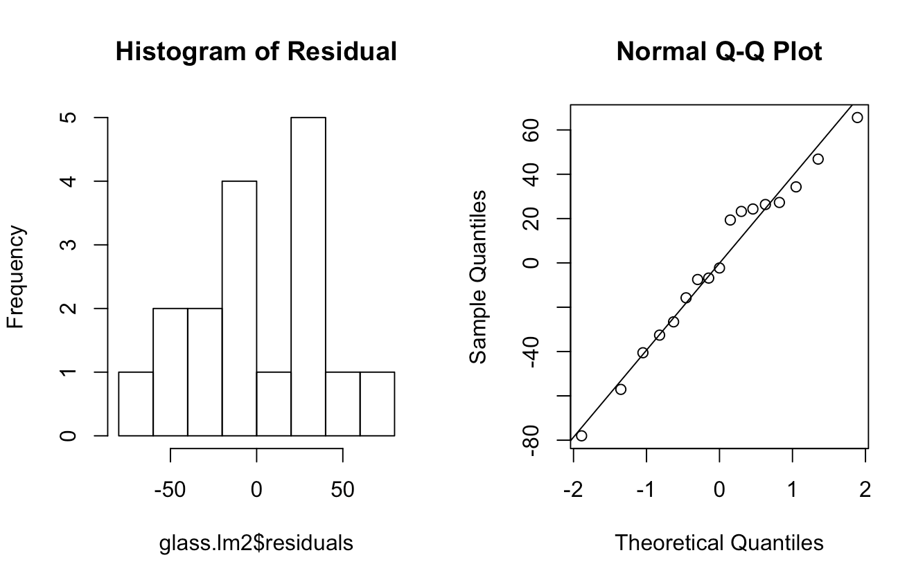
假设3：残差符合正态分布 (normality)

# test for normality
hist(glass.lm2$residuals, main = 'Histogram of Residual')
qqnorm(glass.lm2$residuals)
qqline(glass.lm2$residuals)

# alternative
## dat1 <- as.data.frame(glass.lm2$residuals)
## names(dat1) <- 'res'
## theme_set(
## theme_minimal() +
## theme(legend.position = "top"))
## ggplot(dat1,aes(sample = res)) + stat_qq()

 

# Shapiro–Wilk test
# H0: 样本数据与正态分布没有显著区别。
# HA: 样本数据与正态分布存在显著区别。
shapiro.test(glass.lm2$residuals)

 

 

 

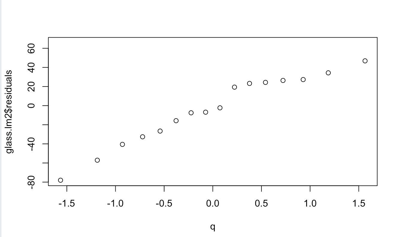
# roughly achieve qqplot by hand 
par(mfrow=c(1,1))
t <- rank(glass.lm2$residuals)/length(glass.lm2$residuals) #求观察累积概率
q <- qnorm(t) #用累积概率求分位数值
plot(q,glass.lm2$residuals)

 

 

 

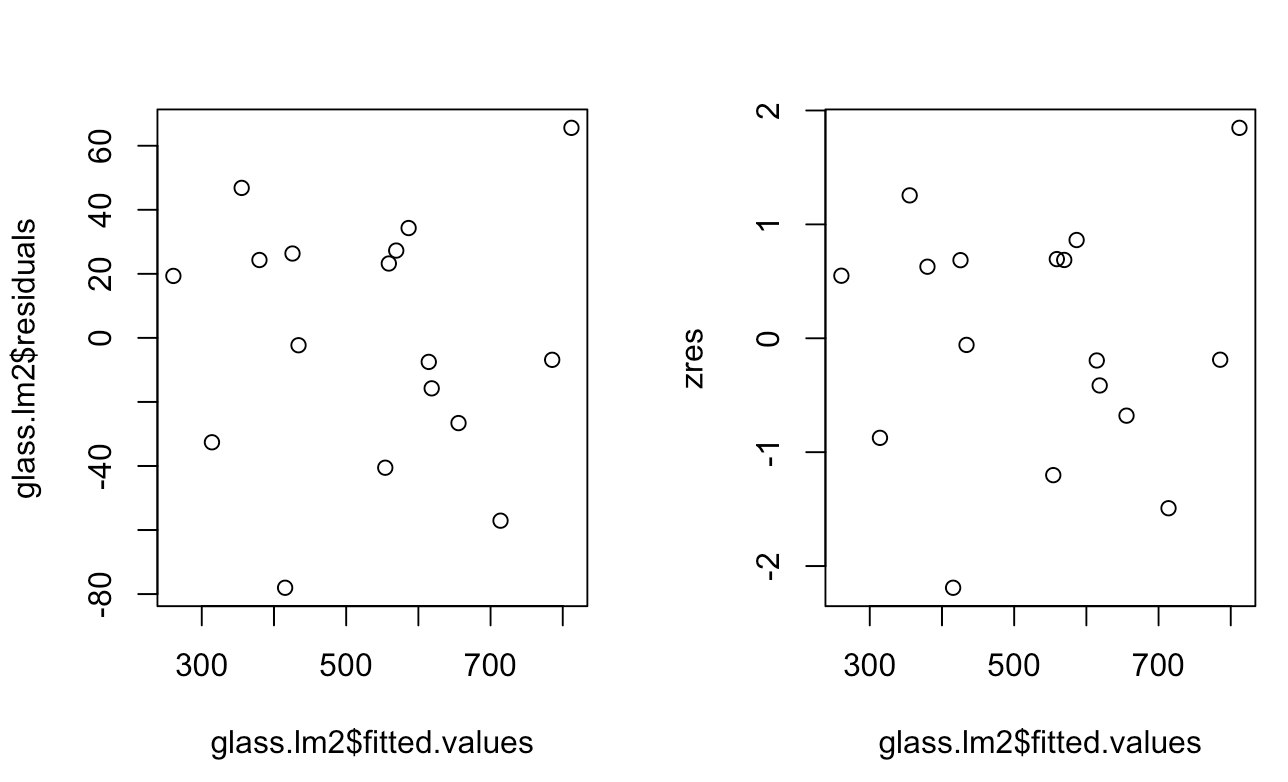
假设4：残差满足同方差性 (homoscedasticity)

# test for homoscedasticity
par(mfrow=c(1,2))
plot(glass.lm2$fitted.values, glass.lm2$residuals)
zres <- rstandard(glass.lm2)
plot(glass.lm2$fitted.values, zres)

 

 

 

假设5： 残差满足独立性 (independence)

# test for independence
par(mfrow=c(1,1))
data <- data.frame(YEAR=c(1:17))
newglassdata <- cbind(glass,data)
#newglassdata
plot(newglassdata$YEAR, glass.lm2$residuals)

 

 

 

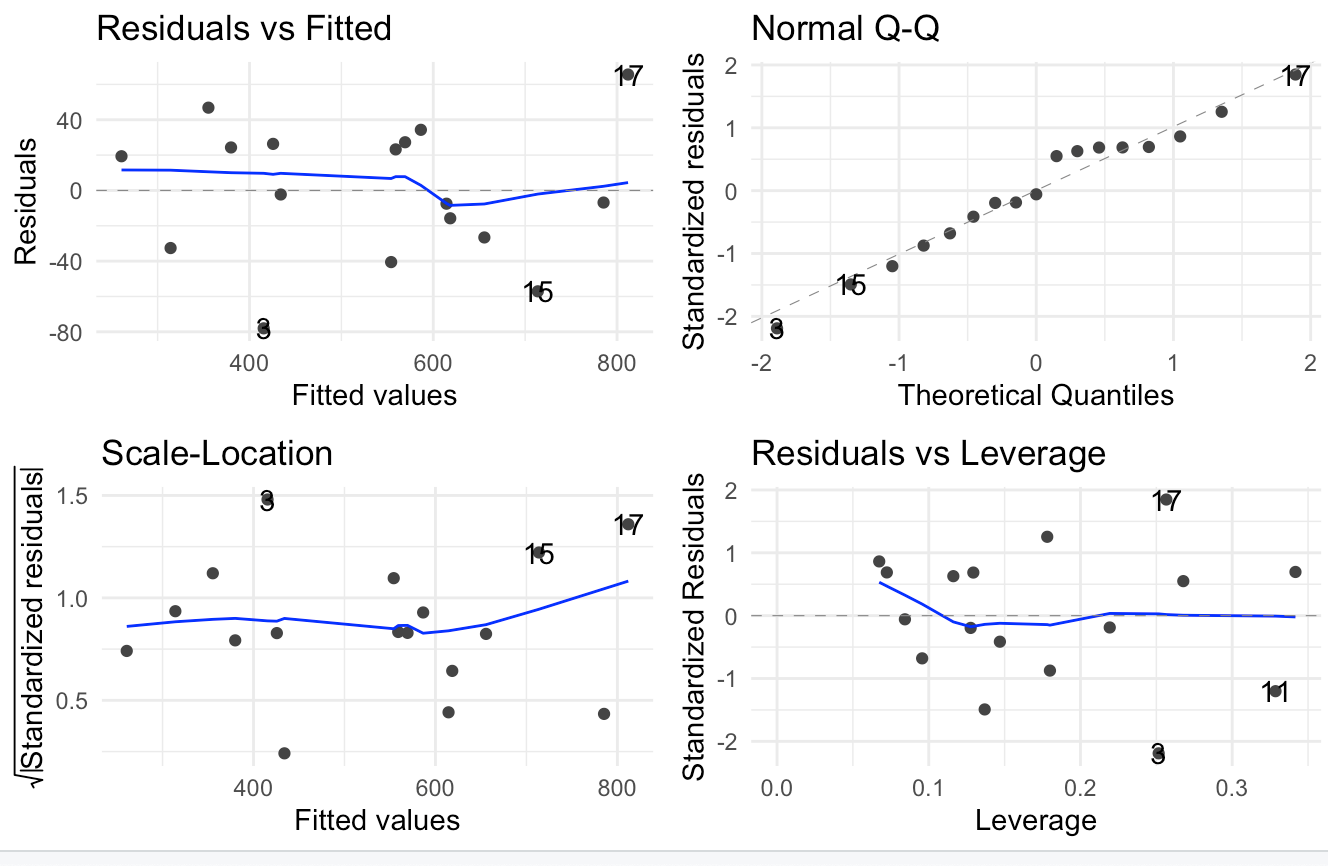
# check model assumption in one step
library(ggfortify)
autoplot(glass.lm2)
# alternative
# par(mfrow = c(2,2))
# plot(glass.lm2)