【R语言学习笔记】8. 非线性模型及交叉检验

 

1. 目的：通过案例介绍R语言实现交叉检验的方法，构建非线性回归模型，并比较不同模型的准确性。

 

2. 数据来源：Datacamp 

https://assets.datacamp.com/production/repositories/894/datasets/6f144237ef9d7da94b2c84aa8eccc519bae4b300/houseprice.rds

 

3. 数据介绍

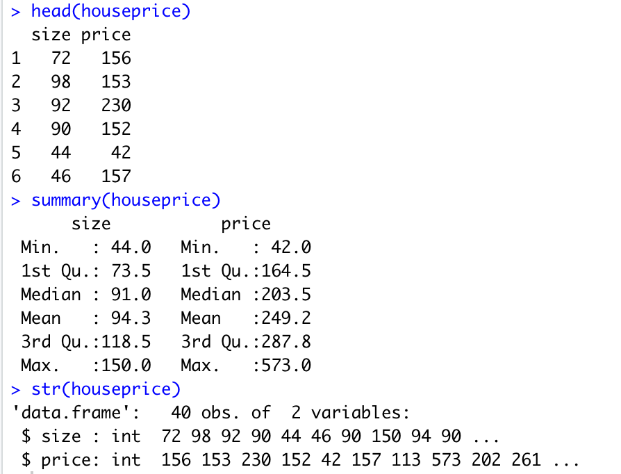
数据中含有40个观测值以及两个变量：房子大小以及房子价格。本文希望通过利用房子大小信息来预测房价信息。

houseprice <- readRDS(gzcon(url("https://assets.datacamp.com/production/repositories/894/datasets/6f144237ef9d7da94b2c84aa8eccc519bae4b300/houseprice.rds")))
head(houseprice)
summary(houseprice)

 

 

 

4. 应用

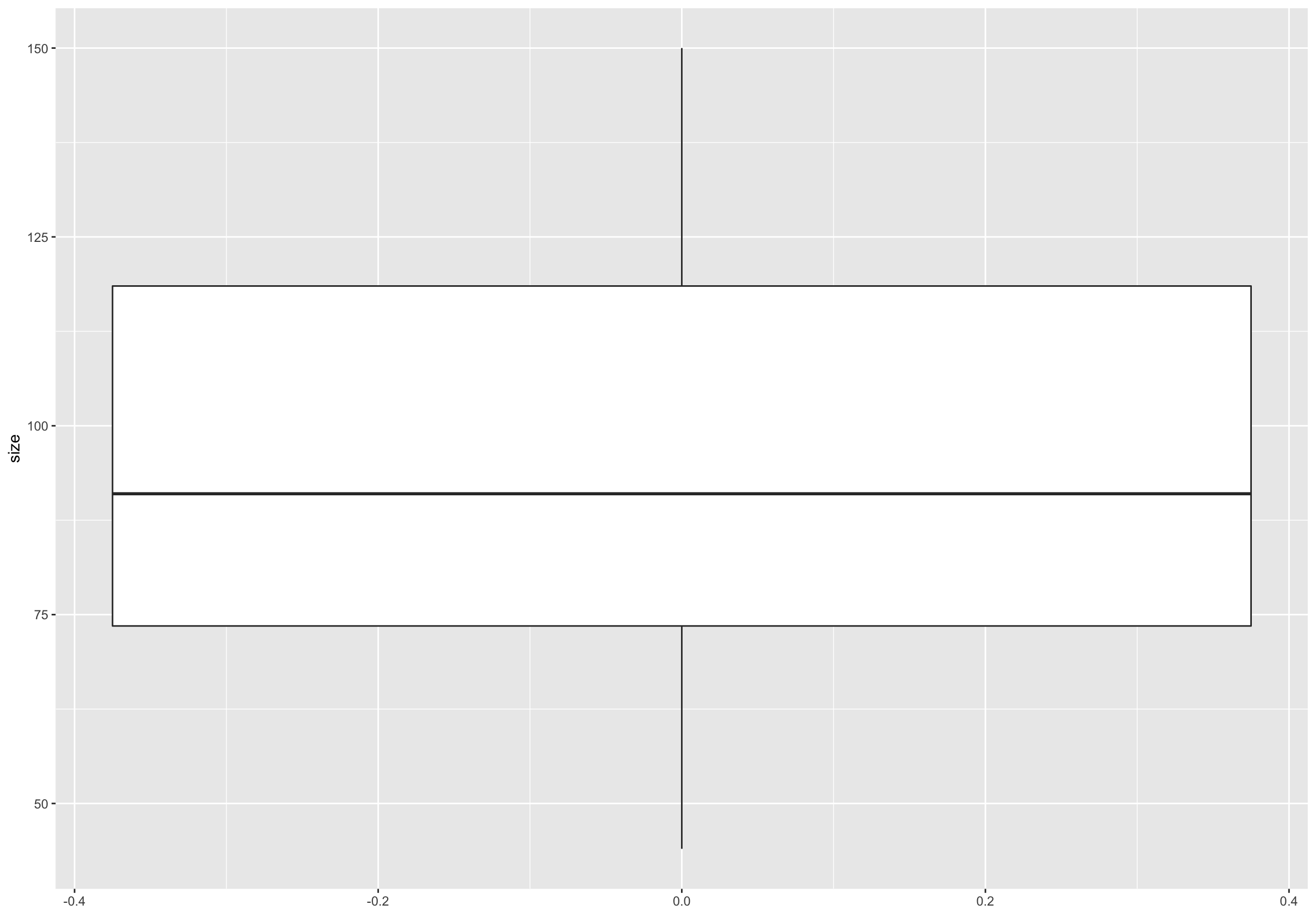
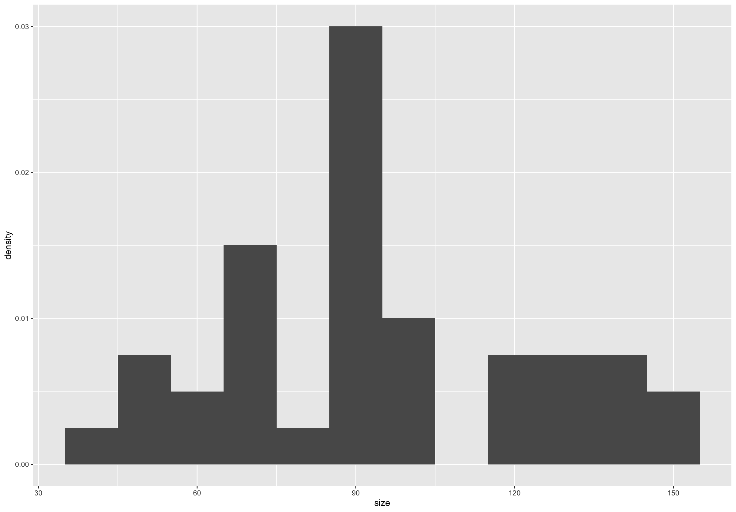
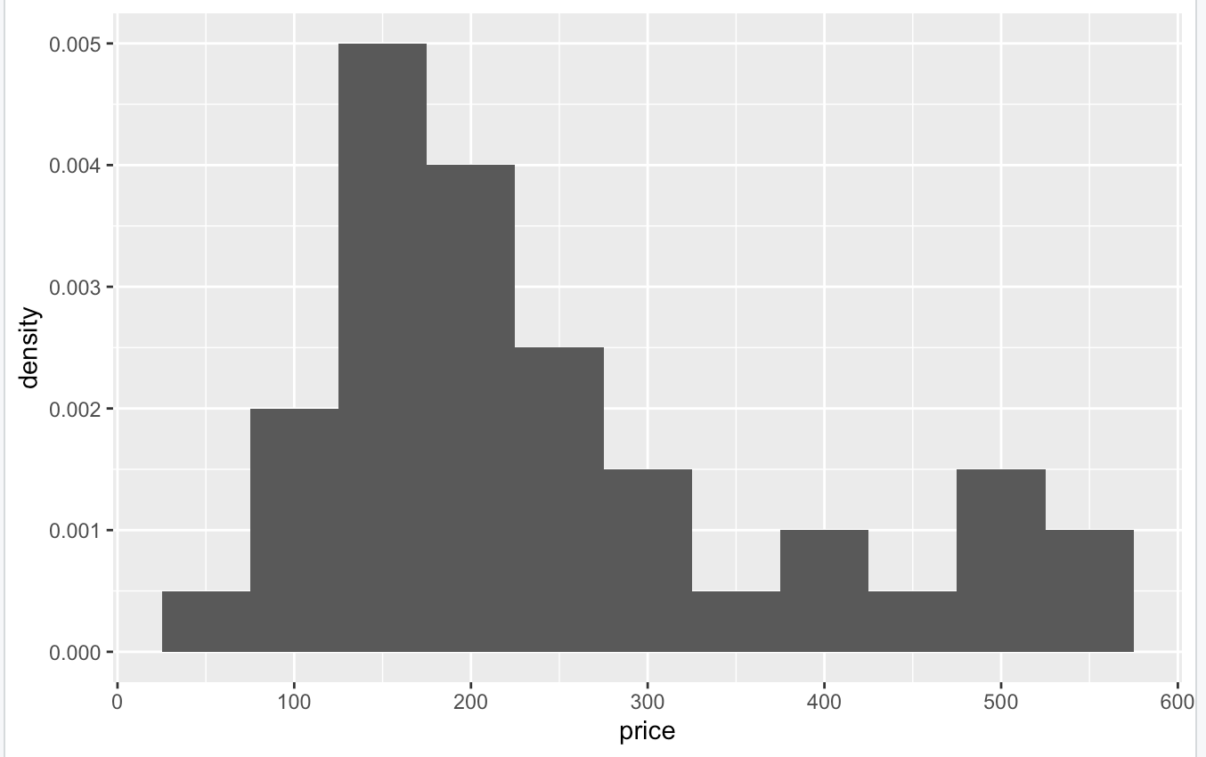
4.1 绘制直方图及箱线图查看变量分布及异常值

# explore the data
library(ggplot2)

# size
ggplot(houseprice, aes(y = size)) + geom_boxplot(outlier.colour = 'darkblue', outlier.shape = 5, outlier.size = 3)
ggplot(houseprice, aes(x = size)) + geom_histogram(aes(y = ..density..), binwidth = 10)

 

 

 

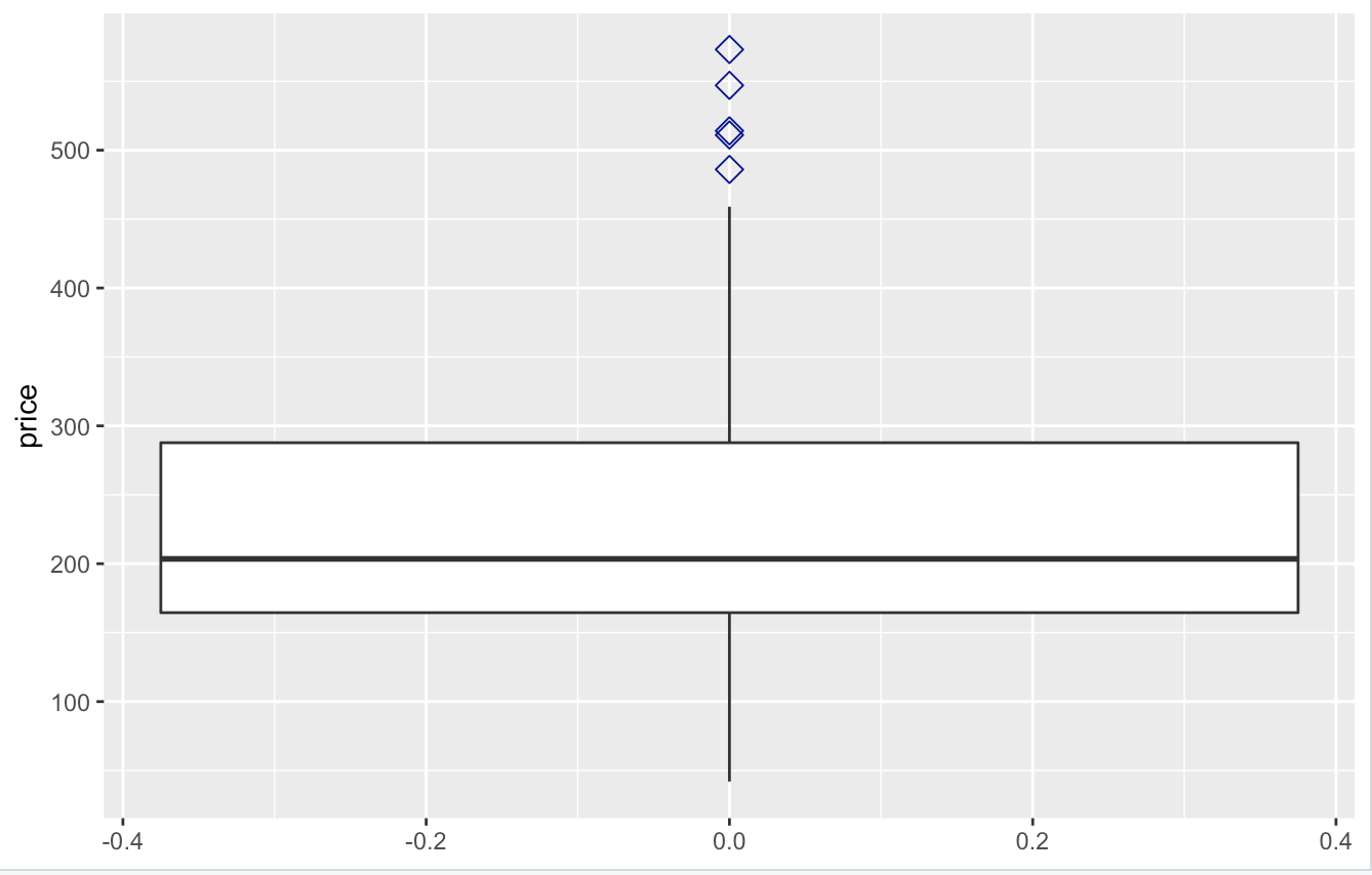
# price
ggplot(houseprice, aes(y = price)) + geom_boxplot(outlier.colour = 'darkblue', outlier.shape = 5, outlier.size = 3)
diff(range(houseprice$price))
ggplot(houseprice, aes(x = price)) + geom_histogram(aes(y = ..density..), binwidth = 50)

 

 

 

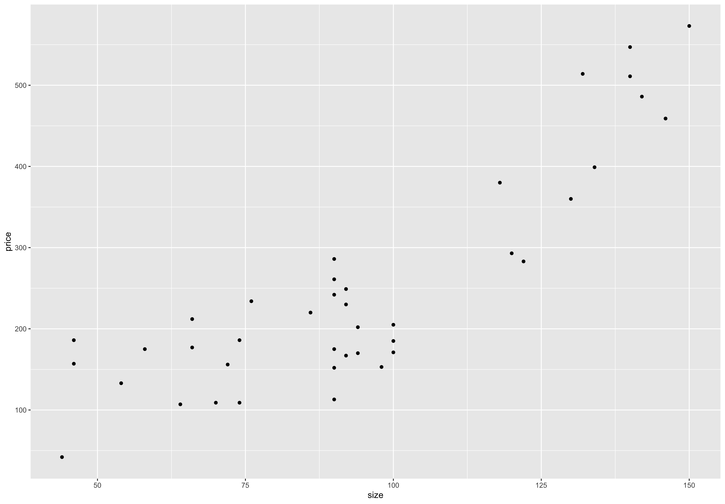
# realtionship b/w size and price
ggplot(houseprice, aes(x = size, y = price)) + geom_point() # non-linear relationship

 

 

4.2 构建模型

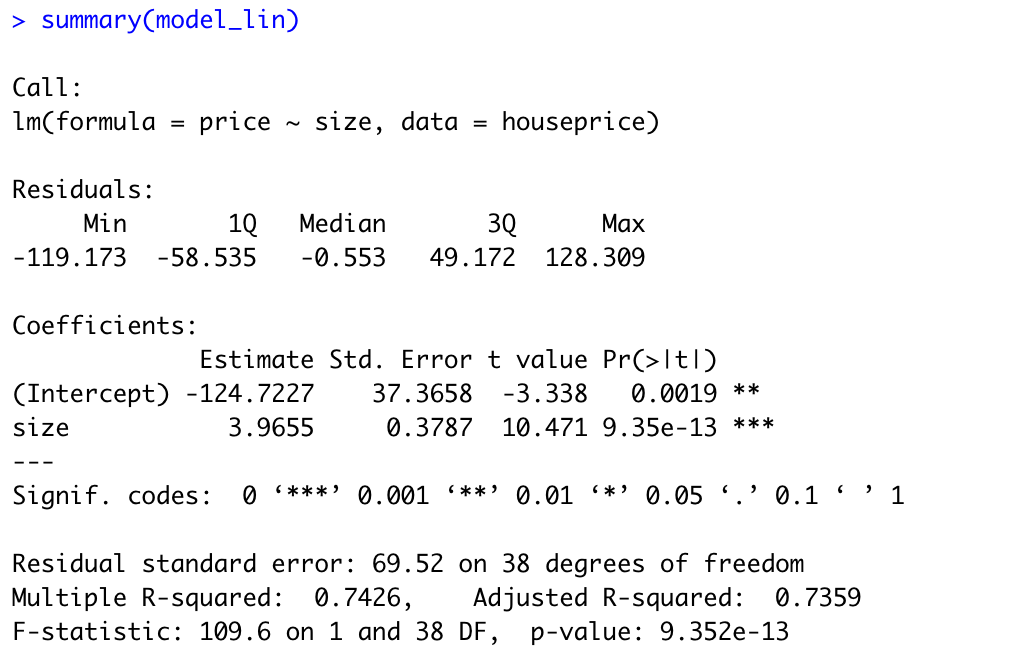
Model1: Linear Regression Model

# Fit a model of price as a linear function of size
model_lin <- lm(price ~ size, houseprice)
summary(model_lin)

 

 

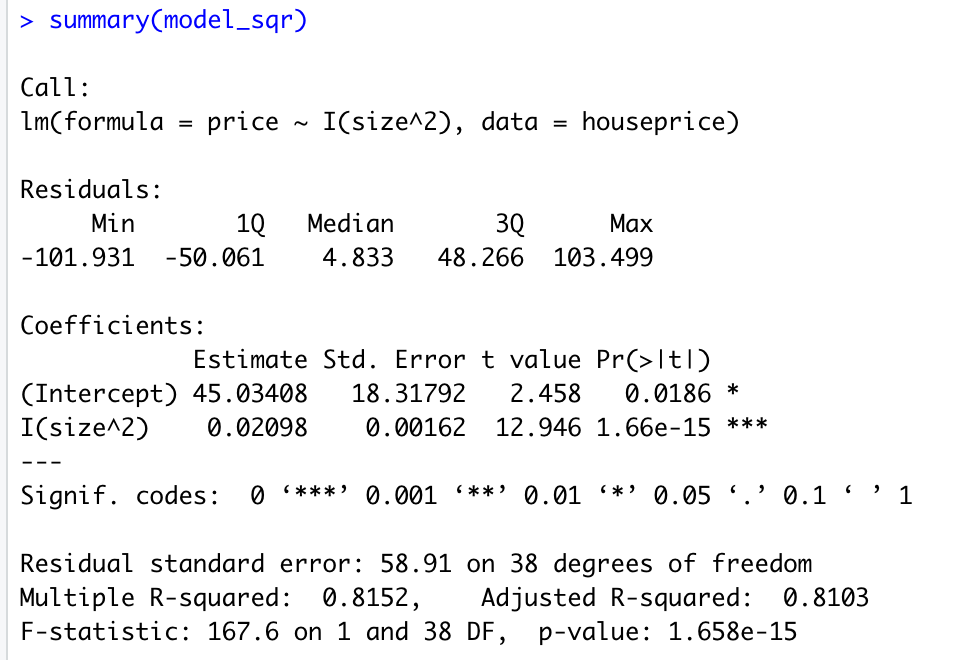
Model2: Quadratic Model

# Fit a model of price as a function of squared size 
model_sqr <- lm(price ~ I(size^2), houseprice)
summary(model_sqr)

 

 

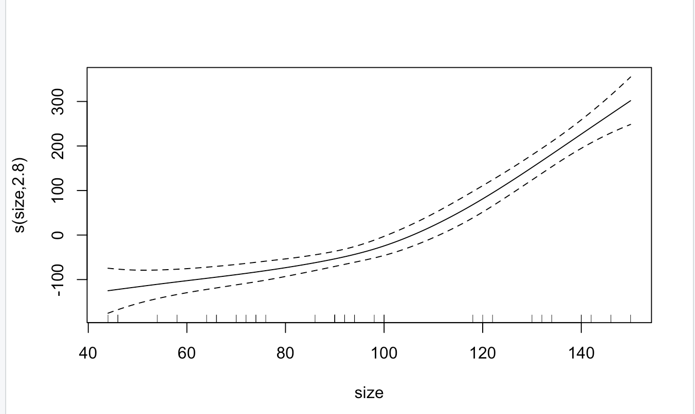
Model3: Generalized Additive Model

library(mgcv)
model_gam <- gam(price ~ s(size), data = houseprice, family = 'gaussian')
summary(model_gam)

 

 

 

plot(model_gam)

 

 

 

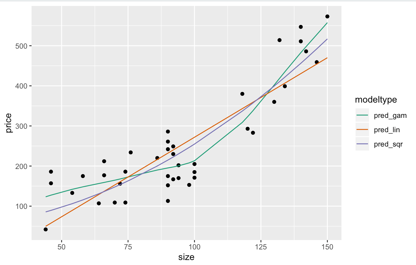
Model comparison

library(dplyr)
library(tidyr)
houseprice %>% 
  mutate(pred_lin = predict(model_lin),       
         pred_sqr = predict(model_sqr),     
         pred_gam = predict(model_gam)) %>%    
  gather(key = modeltype, value = pred, pred_lin, pred_sqr, pred_gam) %>%
  ggplot(aes(x = size)) + 
  geom_point(aes(y = price)) +                   # actual prices
  geom_line(aes(y = pred, color = modeltype)) + # the predictions
  scale_color_brewer(palette = "Dark2")

 

 

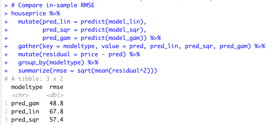
4.3 样本内模型准确性比较(In-Sample RMSE)

# Compare in-sample RMSE
houseprice %>% 
  mutate(pred_lin = predict(model_lin),       
         pred_sqr = predict(model_sqr),     
         pred_gam = predict(model_gam)) %>%    
  gather(key = modeltype, value = pred, pred_lin, pred_sqr, pred_gam) %>%
  mutate(residual = price - pred) %>%
  group_by(modeltype) %>%
  summarize(rmse = sqrt(mean(residual^2)))

 

 

4.4 样本外模型准确性比较(Out-of-Sample RMSE + Cross-Validation)

Cross-Validation Method1

# Create a splitting plan for 3-fold cross validation
library(vtreat)
set.seed(34245)  # set the seed for reproducibility
splitPlan <- kWayCrossValidation(nrow(houseprice), 3, NULL, NULL)

# get cross-validation predictions for price ~ size
houseprice$pred_lin2 <- 0  # initialize the prediction vector
for(i in 1:3) {
  split <- splitPlan[[i]]
  model_lin2 <- lm(price ~ size, data = houseprice[split$train,])
  houseprice$pred_lin2[split$app] <- predict(model_lin2, newdata = houseprice[split$app,])
}

# Get cross-validation predictions for price as a function of size^2 
houseprice$pred_sqr2 <- 0 # initialize the prediction vector
for(i in 1:3) {
  split <- splitPlan[[i]]
  model_sqr2 <- lm(price ~ I(size^2), data = houseprice[split$train, ])
  houseprice$pred_sqr2[split$app] <- predict(model_sqr2, newdata = houseprice[split$app, ])
}

# Get cross-valalidation predictions for price as a function of GAM 
houseprice$pred_gam2 <- 0 # initialize the prediction vector
for(i in 1:3) {
  split <- splitPlan[[i]]
  model_gam2 <- gam(price ~ s(size), data = houseprice[split$train, ])
  houseprice$pred_gam2[split$app] <- predict(model_gam2, newdata = houseprice[split$app, ])
}

 

Cross-Validation Method2 

# alternative for cross validation
library(caret)
myControl <- trainControl(method = "cv", 
                          number = 3,
                          verboseIter = T)
model_lin3 <- train(
  price ~ size, 
  houseprice,
  method = "lm",
  trControl = myControl)

model_sqr3 <- train(
  price ~ I(size^2), 
  houseprice,
  method = "lm",
  trControl = myControl)

model_gam3 <- train(
  price ~ size, 
  houseprice,
  method = "gam",
  trControl = myControl)

model_lin3$results$RMSE
model_sqr3$results$RMSE
model_gam3$results$RMSE

　　

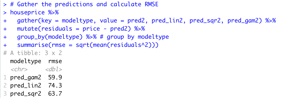
Out-of-Sample  RMSE

# Gather the predictions and calculate RMSE
houseprice %>%
  gather(key = modeltype, value = pred2, pred_lin2, pred_sqr2, pred_gam2) %>%
  mutate(residuals = price - pred2) %>% 
  group_by(modeltype) %>% # group by modeltype
  summarise(rmse = sqrt(mean(residuals^2))

 

  

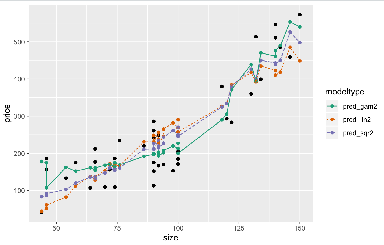
Compare the predictions against actual prices on the data

houseprice %>%
  gather(key = modeltype, value = pred2, pred_lin2, pred_sqr2, pred_gam2) %>%
  ggplot(aes(x = size)) +                          # the column for the x axis
  geom_point(aes(y = price)) +                     # the y-column for the scatterplot
  geom_point(aes(y = pred2, color = modeltype)) +  # the y-column for the point-and-line plot
  geom_line(aes(y = pred2, color = modeltype, linetype = modeltype)) + # the y-column for the point-and-line plot
  scale_color_brewer(palette = "Dark2")