scikit-learn 实现一个基于随机梯度下降的 Logistic回归模型

介绍：用 scikit-learn 库的 SDGClassifier 在 iris 数据集上训练一个基于随机梯度下降的 Logistic回归模型，用事先定义一个可视化分类器模型决策区域的函数在二维图像中绘制决策区域、训练样本和测试样本。

1、可视化决策区域的函数

import numpy as np
import matplotlib.pyplot as plt
from matplotlib.colors import ListedColormap

def plot_decision_regions(X, y, classifier, test_idx=None, resolution=0.02):
    
    # 定义颜色和标记符号，通过颜色列图表生成颜色示例图
    marker = ('o', 'x', 's', 'v', '^')
    colors = ('lightgreen', 'blue', 'red', 'cyan', 'gray')
    cmap = ListedColormap(colors[:len(np.unique(y))])

    # 可视化决策边界
    x1_min, x1_max = X[:, 0].min() - 1, X[:, 0].max() + 1
    x2_min, x2_max = X[:, 1].min() - 1, X[:, 1].max() + 1
    xx1, xx2 = np.meshgrid(np.arange(x1_min, x1_max, resolution),
                           np.arange(x2_min, x2_max, resolution))
    Z = classifier.predict(np.array([xx1.ravel(), xx2.ravel()]).T)
    Z = Z.reshape(xx1.shape)
    
    plt.contourf(xx1, xx2, Z, alpha=0.4, cmap=cmap)
    plt.xlim(xx1.min(), xx1.max())
    plt.ylim(xx2.min(), xx2.max())
    
    # 绘制所有的样本点
    for idx, cl in enumerate(np.unique(y)):
        plt.scatter(x=X[y == cl, 0], y=X[y == cl, 1], alpha=0.8,
                    c=cmap(idx), marker=marker[idx], s=73, label=cl)
    
    # 使用小圆圈高亮显示测试集的样本
    if test_idx:
        X_test, y_test = X[test_idx, :], y[test_idx]
        plt.scatter(X_test[:, 0], X_test[:, 1], c='', alpha=1.0, linewidth=1,
                    edgecolors='black', marker='o', s=135, label='test set')

2、iris 数据处理

from sklearn import datasets
from sklearn.model_selection import train_test_split
from sklearn.preprocessing import StandardScaler

iris = datasets.load_iris()
X = iris.data[:, [2, 3]]
y = iris.target

# 划分测试集和训练集
X_train, X_test, y_train, y_test = train_test_split( 
            X, y, test_size=0.3, random_state=0)

# 对特征值进行标准化
sc = StandardScaler()
sc.fit(X_train)
X_train_std = sc.transform(X_train)
X_test_std = sc.transform(X_test)

3、训练模型，绘制图像

from sklearn.linear_model import SGDClassifier

%matplotlib inline
plt.rcParams['font.sans-serif'] = 'SimHei'
plt.rcParams['axes.unicode_minus'] = False

lr = SGDClassifier(loss='log')
lr.fit(X_train_std, y_train)

# 将标准化后的训练数据和测试数据重新整合到一起
X_combined_std = np.vstack((X_train_std, X_test_std))
y_combined = np.hstack((y_train, y_test))

plt.figure(figsize=(12, 7))
plot_decision_regions(X_combined_std, y_combined, classifier=lr,
                      test_idx=range(105, 150))
plt.title('逻辑斯谛回归模型的决策区域', fontsize=19, color='w')
plt.xlabel('标准化处理后的花瓣长度', fontsize=15)
plt.ylabel('标准化处理后的花瓣宽度', fontsize=15)
plt.legend(loc=2, fontsize=15, scatterpoints=2)

print()

图形：

 

 

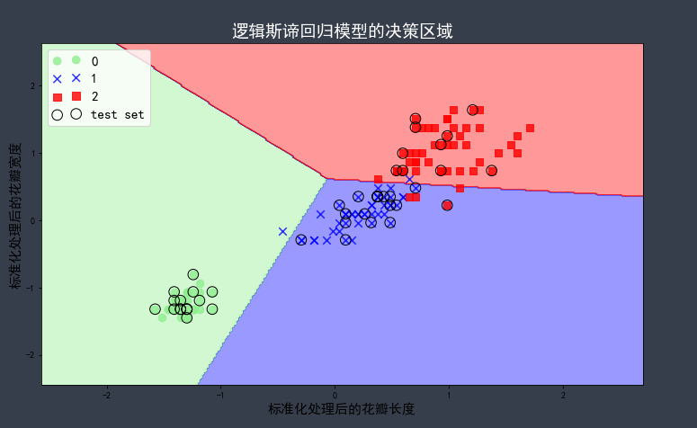
说明：随机梯度下降会产生不同的模型参数，导致决策区域的不同。