ADC and DAC Analog Filters for Data Conversion

Figure 3-7 shows a block diagram of a DSP system, as the sampling theorem dictates it should be.

Before encountering the analog-to-digital converter,

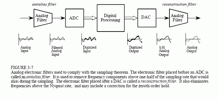
the input signal is processed with an electronic low-pass filter to remove all frequencies above the Nyquist frequency (one-half the sampling rate). This is done to prevent aliasing during sampling, and is correspondingly called an antialias filter. On the other end, the digitized signal is passed through a digital-to-analog converter and another low-pass filter set to the Nyquist frequency. This output filter is called a reconstruction filter, and may include the previously described frequency boost. Unfortunately, there is a serious problem with this simple model: the limitations of electronic filters can be as bad as the problems they are trying to prevent.

If your main interest is in software, you are probably thinking that you don't need to read this section. Wrong! Even if you have vowed never to touch an oscilloscope, an understanding of the properties of analog filters is important for successful DSP. First, the characteristics of every digitized signal you encounter will depend on what type of antialias filter was used when it was acquired. If you don't understand the nature of the antialias filter, you cannot understand the nature of the digital signal. Second, the future of DSP is to replace hardware with software. For example, the multirate techniques presented later in this chapter reduce the need for antialias and reconstruction filters by fancy software tricks. If you don't understand the hardware, you cannot design software to replace it. Third, much of DSP is related to digital filter design. A common strategy is to start with an equivalent analog filter, and convert it into software. Later chapters assume you have a basic knowledge of analog filter techniques.

Three types of analog filters are commonly used: Chebyshev, Butterworth, and Bessel (also called a Thompson filter). Each of these is designed to optimize a different performance parameter. The complexity of each filter can be adjusted by selecting the number ofpoles, a mathematical term that will be discussed in later chapters. The more poles in a filter, the more electronics it requires, and the better it performs. Each of these names describe what the filter does, not a particular arrangement of resistors and capacitors. For example, a six pole Bessel filter can be implemented by many different types of circuits, all of which have the same overall characteristics. For DSP purposes, the characteristics of these filters are more important than how they are constructed. Nevertheless, we will start with a short segment on the electronic design of these filters to provide an overall framework.

Figure 3-8 shows a common building block for analog filter design, the modified Sallen-Key circuit. This is named after the authors of a 1950s paper describing the technique. The circuit shown is a two pole low-pass filter that can be configured as any of the three basic types. Table 3-1 provides the necessary information to select the appropriate resistors and capacitors. For example, to design a 1 kHz, 2 pole Butterworth filter, Table 3-1 provides the parameters: k₁ = 0.1592 and k₂ = 0.586. Arbitrarily selecting R₁ = 10K and C = 0.01uF (common values for op amp circuits), R and R_f can be calculated as 15.95K and 5.86K, respectively. Rounding these last two values to the nearest 1% standard resistors, results in R = 15.8K and R_f = 5.90K All of the components should be 1% precision or better.

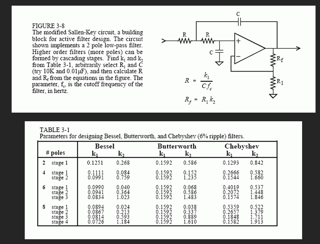
The particular op amp use isn't critical, as long as the unity gain frequency is more than 30 to 100 times higher than the filter's cutoff frequency. This is an easy requirement as long as the filter's cutoff frequency is below about 100 kHz.

Four, six, and eight pole filters are formed by cascading 2,3, and 4 of these circuits, respectively. For example, Fig. 3-9 shows the schematic of a 6 pole

Bessel filter created by cascading three stages. Each stage has different values for k₁ and k₂ as provided by Table 3-1, resulting in different resistors and capacitors being used. Need a high-pass filter? Simply swap the R and C components in the circuits (leaving R_fand R₁ alone).

This type of circuit is very common for small quantity manufacturing and R&D applications; however, serious production requires the filter to be made as an integrated circuit. The problem is, it is difficult to make resistors directly in silicon. The answer is the switched capacitor filter. Figure 3-10 illustrates its operation by comparing it to a simple RC network. If a step function is fed into an RC low-pass filter, the output rises exponentially until it matches the input. The voltage on the capacitor doesn't change instantaneously, because the resistor restricts the flow of electrical charge.

The switched capacitor filter operates by replacing the basic resistor-capacitor network with two capacitors and an electronic switch. The newly added capacitor is much smaller in value than the already existing capacitor, say, 1% of its value. The switch alternately connects the small capacitor between the input and the output at a very high frequency, typically 100 times faster than the cutoff frequency of the filter. When the switch is connected to the input, the small capacitor rapidly charges to whatever voltage is presently on the input. When the switch is connected to the output, the charge on the small capacitor is transferred to the large capacitor. In a resistor, the rate of charge transfer is determined by its resistance. In a switched capacitor circuit, the rate of charge transfer is determined by the value of the small capacitor and by the switching frequency. This results in a very useful feature of switched capacitor

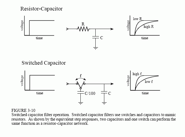
filters: the cutoff frequency of the filter is directly proportional to the clock frequency used to drive the switches. This makes the switched capacitor filter ideal for data acquisition systems that operate with more than one sampling rate. These are easy-to-use devices; pay ten bucks and have the performance of an eight pole filter inside a single 8 pin IC.

Now for the important part: the characteristics of the three classic filter types. The first performance parameter we want to explore iscutoff frequency sharpness. A low-pass filter is designed to block all frequencies above the cutoff frequency (the stopband), while passing all frequencies below (the passband). Figure 3-11 shows the frequency response of these three filters on a logarithmic (dB) scale. These graphs are shown for filters with a one hertz cutoff frequency, but they can be directly scaled to whatever cutoff frequency you need to use. How do these filters rate? The Chebyshev is clearly the best, the Butterworth is worse, and the Bessel is absolutely ghastly! As you probably surmised, this is what the Chebyshev is designed to do, roll-off (drop in amplitude) as rapidly as possible.

Unfortunately, even an 8 pole Chebyshev isn't as good as you would like for an antialias filter. For example, imagine a 12 bit system sampling at 10,000 samples per second. The sampling theorem dictates that any frequency above 5 kHz will be aliased, something you want to avoid. With a little guess work, you decide that all frequencies above 5 kHz must be reduced in amplitude by a factor of 100, insuring that any aliased frequencies will have an amplitude of less than one percent. Looking at Fig. 3-11c, you find that an 8 pole Chebyshev filter, with a cutoff frequency of 1 hertz, doesn't reach an attenuation (signal reduction) of 100 until about 1.35 hertz. Scaling this to the example, the filter's cutoff frequency must be set to 3.7 kHz so that everything above 5 kHz will have the required attenuation. This results in the frequency band between 3.7 kHz and 5 kHz being wasted on the inadequate roll-off of the analog filter.

A subtle point: the attenuation factor of 100 in this example is probably sufficient even though there 4096 steps in 12 bit. From Fig. 3-4, 5100 hertz will alias to 4900 hertz, 6000 hertz will alias to 4000 hertz, etc. You don't care what the amplitudes of the signals between 5000 and 6300 hertz are, because they alias into the unusable region between 3700 hertz and 5000 hertz. In order for a frequency to alias into the filter's passband (0 to 3.7 kHz), it must be greater than 6300 hertz, or 1.7 times the filter's cutoff frequency of 3700 hertz. As shown in Fig. 3-11c, the attenuation provided by an 8 pole Chebyshev filter at 1.7 times the cutoff frequency is about 1300, much more adequate than the 100 we started the analysis with. The moral to this story: In most systems, the frequency band between about 0.4 and 0.5 of the sampling frequency is an unusable wasteland of filter roll-off and aliased signals. This is a direct result of the limitations of analog filters.

The frequency response of the perfect low-pass filter is flat across the entire passband. All of the filters look great in this respect in Fig. 3-11, but only because the vertical axis is displayed on a logarithmic scale. Another story is told when the graphs are converted to alinear vertical scale, as is shown

in Fig. 3-12. Passband ripple can now be seen in the Chebyshev filter (wavy variations in the amplitude of the passed frequencies). In fact, the Chebyshev filter obtains its excellent roll-off by allowing this passband ripple. When more passband ripple is allowed in a filter, a faster roll-off can be achieved. All the Chebyshev filters designed by using Table 3-1 have a passband ripple of about 6% (0.5 dB), a good compromise, and a common choice. A similar design, the elliptic filter, allows ripple in both the passband and the stopband. Although harder to design, elliptic filters can achieve an even better tradeoff between roll-off and passband ripple.

In comparison, the Butterworth filter is optimized to provide the sharpest roll-off possible without allowing ripple in the passband. It is commonly called the maximally flat filter, and is identical to a Chebyshev designed for zero passband ripple. The Bessel filter has no ripple in the passband, but the roll-off far worse than the Butterworth.

The last parameter to evaluate is the step response, how the filter responds when the input rapidly changes from one value to another. Figure 3-13 shows the step response of each of the three filters. The horizontal axis is shown for filters with a 1 hertz cutoff frequency, but can be scaled (inversely) for higher cutoff frequencies. For example, a 1000 hertz cutoff frequency would show a step response inmilliseconds, rather than seconds. The Butterworth and Chebyshev filters overshoot and show ringing (oscillations that slowly decreasing in amplitude). In comparison, the Bessel filter has neither of these nasty problems.

 

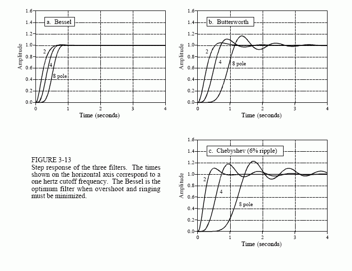
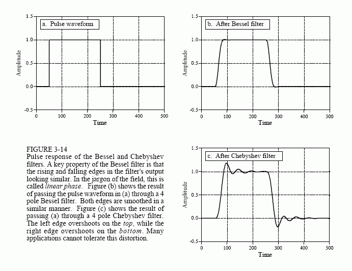
Figure 3-14 further illustrates this very favorable characteristic of the Bessel filter. Figure (a) shows a pulse waveform, which can be viewed as a rising step followed by a falling step. Figures (b) and (c) show how this waveform

would appear after Bessel and Chebyshev filters, respectively. If this were a video signal, for instance, the distortion introduced by the Chebyshev filter would be devastating! The overshoot would change the brightness of the edges of objects compared to their centers. Worse yet, the left side of objects would look bright, while the right side of objects would look dark. Many applications cannot tolerate poor performance in the step response. This is where the Bessel filter shines; no overshoot and symmetrical edges.

 

Next Section: Selecting The Antialias Filter

Table 3-2 summarizes the characteristics of these three filters, showing how each optimizes a particular parameter at the expense of everything else. The Chebyshev optimizes the roll-off, the Butterworth optimizes the passband flatness, and the Bessel optimizes thestep response.

The selection of the antialias filter depends almost entirely on one issue: how information is represented in the signals you intend to process. While 

there are many ways for information to be encoded in an analog waveform, only two methods are common, time domain encoding, and frequency domain encoding. The difference between these two is critical in DSP, and will be a reoccurring theme throughout this book.

In frequency domain encoding, the information is contained in sinusoidal waves that combine to form the signal. Audio signals are an excellent example of this. When a person hears speech or music, the perceived sound depends on the frequencies present, and not on the particular shape of the waveform. This can be shown by passing an audio signal through a circuit that changes the phase of the various sinusoids, but retains their frequency and amplitude. The resulting signal looks completely different on an oscilloscope, butsounds identical. The pertinent information has been left intact, even though the waveform has been significantly altered. Since aliasing misplaces and overlaps frequency components, it directly destroys information encoded in the frequency domain. Consequently, digitization of these signals usually involves an antialias filter with a sharp cutoff, such as a Chebyshev, Elliptic, or Butterworth. What about the nasty step response of these filters? It doesn't matter; the encoded information isn't affected by this type of distortion.

In contrast, time domain encoding uses the shape of the waveform to store information. For example, physicians can monitor the electrical activity of a person's heart by attaching electrodes to their chest and arms (an electrocardiogram or EKG). The shape of the EKG waveform provides the information being sought, such as when the various chambers contract during a heartbeat. Images are another example of this type of signal. Rather than a waveform that varies over time, images encode information in the shape of a waveform that varies over distance. Pictures are formed from regions of brightness and color, and how they relate to other regions of brightness and color. You don't look at the Mona Lisa and say, "My, what an interesting collection of sinusoids."

Here's the problem: The sampling theorem is an analysis of what happens in the frequency domain during digitization. This makes it ideal to under-stand the analog-to-digital conversion of signals having their information encoded in the frequency domain. However, the sampling theorem is little help in understanding how time domain encoded signals should be digitized. Let's take a closer look.

Figure 3-15 illustrates the choices for digitizing a time domain encoded signal. Figure (a) is an example analog signal to be digitized. In this case, the information we want to capture is the shape of the rectangular pulses. A short burst of a high frequency sine wave is also included in this example signal. This represents wideband noise, interference, and similar junk that always appears on analog signals. The other figures show how the digitized signal would appear with different antialias filter options: a Chebyshev filter, a Bessel filter, and no filter.

It is important to understand that none of these options will allow the original signal to be reconstructed from the sampled data. This is because the original signal inherently contains frequency components greater than one-half of the sampling rate. Since these frequencies cannot exist in the digitized signal, the reconstructed signal cannot contain them either. These high frequencies result from two sources: (1) noise and interference, which you would like to eliminate, and (2) sharp edges in the waveform, which probably contain information you want to retain.

The Chebyshev filter, shown in (b), attacks the problem by aggressively removing all high frequency components. This results in a filtered analog signal that can be sampled and later perfectly reconstructed. However, the reconstructed analog signal is identical to thefiltered signal, not the original signal. Although nothing is lost in sampling, the waveform has been severely distorted by the antialias filter. As shown in (b), the cure is worse than the disease! Don't do it!

The Bessel filter, (c), is designed for just this problem. Its output closely resembles the original waveform, with only a gentle rounding of the edges. By adjusting the filter's cutoff frequency, the smoothness of the edges can be traded for elimination of high frequency components in the signal. Using more poles in the filter allows a better tradeoff between these two parameters. A common guideline is to set the cutoff frequency at about one-quarter of the sampling frequency. This results in about two samples along the rising portion of each edge. Notice that both the Bessel and the Chebyshev filter have removed the burst of high frequency noise present in the original signal.

The last choice is to use no antialias filter at all, as is shown in (d). This has the strong advantage that the value of each sample isidentical to the value of the original analog signal. In other words, it has perfect edge sharpness; a change in the original signal is immediately mirrored in the digital data. The disadvantage is that aliasing can distort the signal. This takes two different forms. First, high frequency interference and noise, such as the example sinusoidal burst, will turn into meaningless samples, as shown in (d). That is, any high frequency noise present in the analog signal will appear as aliased noise in the digital signal. In a more general sense, this is not a problem of the sampling, but a problem of the upstream analog electronics. It is not the ADC's purpose to reduce noise and interference; this is the responsibility of the analog electronics before the digitization takes place. It may turn out that a Bessel filter should be placed before the digitizer to control this problem. However, this means the filter should be viewed as part of the analog processing, not something that is being done for the sake of the digitizer.

The second manifestation of aliasing is more subtle. When an event occurs in the analog signal (such as an edge), the digital signal in (d) detects the change on the next sample. There is no information in the digital data to indicate what happens between samples. Now, compare using no filter with using a Bessel filter for this problem. For example, imagine drawing straight lines between the samples in (c). The time when this constructed line crosses one-half the amplitude of the step provides a subsample estimate of when the edge occurred in the analog signal. When no filter is used, this subsample information is completely lost. You don't need a fancy theorem to evaluate how this will affect your particular situation, just a good understanding of what you plan to do with the data once is it acquired.