Python机器学习2.2

使用Python实现感知器学习算法

 在《Python机器学习》中的2.2节中，创建了罗森布拉特感知器的类，通过fit方法初始化权重self.w_，再fit方法循环迭代样本，更新权重，使用predict方法计算类标，将每轮迭代中错误分类样本的数量存放于列表self.errors_中。罗森布拉特感知器可以参考这个网址或自行百度。https://www.jb51.net/article/130970.htm

import numpy as np
class Perceptron(object):
    """感知器分类器.
    
    参数
    ----------
    eta(学习速率) : float
        学习率（介于0和1之间）
    n_iter(迭代次数) : int
        通过训练数据集.
        
    属性
    ----------
    w_ : id-array
        fit方法后的权重.
    errors_ : list
        每轮迭代错误分类样本的数量存放列表.
        
    """
    def __init__(self, eta=0.01, n_iter=10):
        self.eta = eta
        self.n_iter = n_iter
        
    def fit(self, X, y):
        """拟合训练数据.
        
        参数
        ----------
        X : {array-like}, shape = {n_samples, n_features}
            训练向量, 其中n_samples是样本的数目,
            n_features是特征的数目(维数).
        y : array-like, shape = {n_samples}
            目标值.
            
            返回
        ----------
        self : object
        
        """
        self.w_ = np.zeros(1 + X.shape[1])
        self.errors_ = []
        
        for _ in range(self.n_iter):
            errors = 0
            for xi, target in zip(X, y):
                update = self.eta * (target - self.predict(xi))
                self.w_[1:] += update * xi
                self.w_[0] += update
                errors += int(update != 0.0)
            self.errors_.append(errors)
        return self
    
    def net_input(self, X):
        """Calculate net input"""
        return np.dot(X, self.w_[1:]) + self.w_[0]
    
    def predict(self, X):
        """每一步后返回类标签"""
        return np.where(self.net_input(X) >= 0.0, 1, -1)

 

书中选用了鸢尾花数据集中的山鸢尾(Setosa)和变色鸢尾(Versicolor)俩种信息作为测试数据。出于可视化，选取了萼片长度(sepal length)和花瓣长度(petal-length)两个特征。

使用pandas库直接从UCI机器学习库中获取鸢尾花数据集(iris.data)并转换为DataFrame对象加载到内存中，使用tail方法显示数据确保正确加载。

import pandas as pd
df = pd.read_csv('https://archive.ics.uci.edu/ml/'
                'machine-learning-databases/iris/iris.data', header=None)
df.tail()

 

提取前100个类标，其中山鸢尾(Setosa)和变色鸢尾(Versicolor)各50个，并将类标用两个整数表示：1表示变色鸢尾，-1表示山鸢尾，赋给NumPy的向量y。类似的，提取前100个训练样本的第一个特征列()和第三个特征列()，赋给X。用二位散点图进行可视化。

import matplotlib.pyplot as plt
import numpy as np
#jupyter notebook显示图片
%matplotlib inline
#中文字体显示  
plt.rc('font', family='SimHei', size=13)

y = df.iloc[0:100, 4].values
y = np.where(y == 'Iris-setosa', -1, 1)
X = df.iloc[0:100, [0,2]].values
plt.scatter(X[:50, 0], X[:50, 1],
           color='red', marker='o', label='setosa')
plt.scatter(X[50:100, 0], X[50:100, 1],
           color='blue', marker='x', label='versicolor')
plt.xlabel('花瓣长度(cm)')
plt.ylabel('萼片长度(cm)')
plt.legend(loc='upper left')
plt.show()

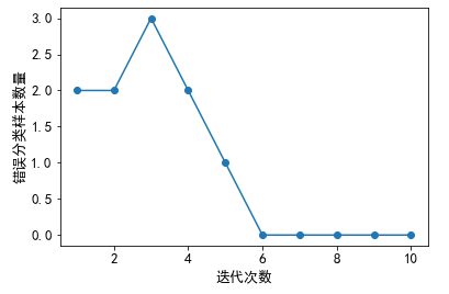
利用抽取的鸢尾花数据子集训练感知器。绘制每次迭代错误分类数量的折线图。

ppn = Perceptron(eta=0.1, n_iter=10)
ppn.fit(X, y)
plt.plot(range(1, len(ppn.errors_) + 1), ppn.errors_,
        marker='o')
plt.xlabel('迭代次数')
plt.ylabel('错误分类样本数量')
plt.show()

 

 

待续。。。