Word2Vec--gensim

本文章参考来自于gensim官方文档 https://radimrehurek.com/gensim/auto_examples/tutorials/run_word2vec.html#sphx-glr-auto-examples-tutorials-run-word2vec-py

word2vec作为基于神经网络的机器学习算法“新潮”的一员，通常被称为“深度学习”（尽管word2vec本身很浅），因此被广泛推荐。使用大量未注释的纯文本，word2vec会自动学习单词之间的关系。输出是向量，每个单词一个向量，具有显着的线性关系，使我们可以执行以下操作

• vec(“king”) - vec(“man”) + vec(“woman”) =~ vec(“queen”)

• vec(“Montreal Canadiens”) – vec(“Montreal”) + vec(“Toronto”) =~ vec(“Toronto Maple Leafs”).

Word2vec在自动文本标记，推荐系统和机器翻译中非常有用。

回顾：词袋¶

如果您已经熟悉模型，可以随时跳过这些检查部分。

该模型将每个文档转换为固定长度的整数矢量。例如，给定句子：

• John likes to watch movies. Mary likes movies too.

• John also likes to watch football games. Mary hates football.

模型输出向量：

• [1, 2, 1, 1, 2, 1, 1, 0, 0, 0, 0]

• [1, 1, 1, 1, 0, 1, 0, 1, 2, 1, 1]

每个向量有10个元素，其中每个元素计算文档中特定单词出现的次数。元素的顺序是任意的。在上面的示例中，元素的顺序对应于单词： 。["John", "likes", "to", "watch", "movies", "Mary", "too", "also", "football", "games", "hates"]

词袋模型出奇地有效，但有几个缺点：

首先，他们会丢失所有有关单词顺序的信息： “John likes Mary” 和 “Mary likes John” 对应于相同的向量。有一个解决方案：bag of n-grams models考虑长度为n的词组来将文档表示为固定长度的向量，以捕获本地词序，但存在数据稀疏和高维的问题。

其次，该模型不会尝试学习基础单词的含义，因此，向量之间的距离并不总是反映出含义上的差异。该Word2Vec模型解决了第二个问题。

介绍：Word2Vec模型

Word2Vec是一种较新的模型，该模型使用浅层神经网络将单词嵌入到低维向量空间中。结果是一组词向量，其中在向量空间中靠在一起的向量根据上下文具有相似的含义，而彼此远离的词向量具有不同的含义。例如，strong和powerful将彼此靠近，strong并且Paris将相对较远。

该模型有两个版本，并且Word2Vec 类同时实现了这两个版本：

1. 跳过码（SG）

2. 连续词袋（CBOW）

Word2Vec Demo

中文词向量数据集https://github.com/RomanGao/Chinese-Word-Vectors

word2vec-google-news-300.gz 链接：https://pan.baidu.com/s/1qEoMqJDBOMYXDPHq7hsDMQ  提取码：mj5j 

我们将获取在Google新闻数据集的一部分上训练的Word2Vec模型，该模型涵盖大约300万个单词和短语。这样的模型可能需要花费数小时来训练，但是由于已经可用，因此使用Gensim进行下载和加载需要几分钟。

您也可以查看在线word2vec演示，在这里可以自己尝试使用矢量代数。该演示程序word2vec在 整个 Google新闻数据集（约1000亿字）上运行。

import gensim.downloader as api
wv = api.load('word2vec-google-news-300')

常见的操作是检索模型的词汇表。这很简单：

for i, word in enumerate(wv.vocab):
    if i == 10:
        break
    print(word)

我们可以轻松获得模型熟悉的术语的向量：

vec_king = wv['king']

出：

</s>
in
for
that
is
on
##
The
with

不幸的是，该模型无法推断出陌生单词的向量。这是Word2Vec的一个限制：如果您对此限制很重要，请查看FastText模型。

try:
    vec_cameroon = wv['cameroon']
except KeyError:
    print("The word 'cameroon' does not appear in this model")　

出： The word 'cameroon' does not appear in this model

继续，Word2Vec开箱即用地支持几个单词相似性任务

pairs = [
    ('car', 'minivan'),   # a minivan is a kind of car
    ('car', 'bicycle'),   # still a wheeled vehicle
    ('car', 'airplane'),  # ok, no wheels, but still a vehicle
    ('car', 'cereal'),    # ... and so on
    ('car', 'communism'),
]
for w1, w2 in pairs:
    print('%r\t%r\t%.2f' % (w1, w2, wv.similarity(w1, w2)))

出：

'car'   'minivan'       0.69
'car'   'bicycle'       0.54
'car'   'airplane'      0.42
'car'   'cereal'        0.14
'car'   'communism'     0.06

打印与“ car”或“ minivan”最相似的5个词

print(wv.most_similar(positive=['car', 'minivan'], topn=5))

出：

[('SUV', 0.853219211101532), ('vehicle', 0.8175784349441528), ('pickup_truck', 0.7763689160346985), ('Jeep', 0.7567334175109863), ('Ford_Explorer', 0.756571888923645)]

以下哪个不属于该顺序？

print(wv.doesnt_match(['fire', 'water', 'land', 'sea', 'air', 'car']))

出：

/home/misha/git/gensim/gensim/models/keyedvectors.py:877: FutureWarning: arrays to stack must be passed as a "sequence" type such as list or tuple. Support for non-sequence iterables such as generators is deprecated as of NumPy 1.16 and will raise an error in the future.
  vectors = vstack(self.word_vec(word, use_norm=True) for word in used_words).astype(REAL)
car

训练你自己的模型

首先，您需要一些数据来训练模型。对于以下示例，我们将使用Lee Corpus （如果已安装gensim，则已经拥有）。

这个语料库足够小，可以完全容纳在内存中，但是我们将实现一个内存友好的迭代器，该迭代器逐行读取它，以演示如何处理更大的语料库

from gensim.test.utils import datapath
from gensim import utils

class MyCorpus(object):
    """An interator that yields sentences (lists of str)."""

    def __iter__(self):
        corpus_path = datapath('lee_background.cor')
        for line in open(corpus_path):
            # assume there's one document per line, tokens separated by whitespace
            yield utils.simple_preprocess(line)

如果我们想进行任何自定义的预处理，例如解码非标准编码，小写字母，删除数字，提取命名实体……所有这些都可以在MyCorpus迭代器内完成，word2vec而无需知道。所需要做的就是输入产生句子迭代器（utf-8的单词列表）。在此处一定是单词列表,比如两句话表示为 [['i', 'hate', 'you'], ['but' ,'i', 'want', 'you']]

 让我们继续，在我们的语料库上训练模型。暂时不必担心训练参数，我们稍后将对其进行重新讨论。

import gensim.models

sentences = MyCorpus()
model = gensim.models.Word2Vec(sentences=sentences)

建立模型后，我们可以使用与上面演示相同的方法。

该模型的主要部分是model.wv，其中“ wv”代表“单词向量”。

vec_king = model.wv['king']

检索词汇的方法相同（wv.vocab 代表这个词）：

for i, word in enumerate(model.wv.vocab):
    if i == 10:
        break
    print(word)

出：

hundreds
of
people
have
been
forced
to
their
homes
in

存储和加载模型

您会注意到，训练non-trivial模型会花费时间。训练好模型并按预期工作后，可以将其保存到磁盘。这样一来，您不必在以后再花时间进行训练。

您可以使用标准gensim方法存储/加载模型：

import tempfile

with tempfile.NamedTemporaryFile(prefix='gensim-model-', delete=False) as tmp:
    temporary_filepath = tmp.name
    model.save(temporary_filepath)
    #
    # The model is now safely stored in the filepath.
    # You can copy it to other machines, share it with others, etc.
    #
    # To load a saved model:
    #
    new_model = gensim.models.Word2Vec.load(temporary_filepath)

它在内部使用pickle，可以选择mmap直接从磁盘文件将模型的内部大型NumPy矩阵“虚拟”到虚拟内存中，以实现进程间内存共享。

此外，您可以使用原始C工具使用其文本格式和二进制格式来加载模型：

 

model = gensim.models.KeyedVectors.load_word2vec_format('/tmp/vectors.txt', binary=False)
# using gzipped/bz2 input works too, no need to unzip
model = gensim.models.KeyedVectors.load_word2vec_format('/tmp/vectors.bin.gz', binary=True)

训练参数

Word2Vec 接受几个影响训练速度和质量的参数。

min_count 

min_count用于修剪内部字典。在十亿个单词的语料库中仅出现一次或两次的单词可能是无趣的错别字和垃圾。此外，没有足够的数据来对这些单词进行任何有意义的训练，因此最好忽略它们：

min_count = 5的默认值

model = gensim.models.Word2Vec(sentences, min_count=10)

size

size 是gensim Word2Vec将单词映射到的N维空间的维数（N）。

较大的值需要更多的训练数据，但可以产生更好（更准确）的模型。合理的值在数十到数百之间。

# default value of size=100
model = gensim.models.Word2Vec(sentences, size=200)

workers

workers，最后一个主要参数（此处完整列表）用于训练并行化，以加快训练速度：

# default value of workers=3 (tutorial says 1...)
model = gensim.models.Word2Vec(sentences, workers=4)

该workers参数仅在安装了Cython后才有效。如果没有用Cython，你只可以使用一个核心因为GIL（和word2vec 训练收敛非常慢）。

内存

在其核心，word2vec模型参数存储为矩阵（NumPy数组）。每个数组是#vocabulary（由min_count参数控制）乘以#size（大小参数）的浮点数（单精度，即4个字节）。

RAM中保存了三个这样的矩阵（正在努力将该数目减少到两个，甚至一个）。因此，如果您的输入包含100,000个唯一的单词，并且您要求layer size=200，则该模型将需要大约。100,000*200*4*3 bytes = ~229MB

存储词汇树需要一点额外的内存（100,000个单词将花费几兆字节），但是除非您的单词是非常宽松的字符串，否则内存占用量将由上述三个矩阵控制。

评估

Word2Vec训练是一项无人监督的任务，没有一种很好的方法可以客观地评估结果。评估取决于您的最终应用。

Gensim以完全相同的格式支持相同的评估集：

model.accuracy('./datasets/questions-words.txt')

这accuracy带有一个可选参数 restrict_vocab，该参数限制要考虑的测试示例。

在2016年12月发布的Gensim中，我们添加了一种更好的方法来评估语义相似性。

默认情况下，它使用学术数据集WS-353，但是可以基于它创建针对您的企业的数据集。它包含单词对以及人类指定的相似性判断。它测量两个单词的相关性或同时出现。

model.evaluate_word_pairs(datapath('wordsim353.tsv'))

Online training / Resuming training

高级用户可以加载模型并继续使用更多的句子和新的词汇量对其进行训练：

model = gensim.models.Word2Vec.load(temporary_filepath)
more_sentences = [
    ['Advanced', 'users', 'can', 'load', 'a', 'model',
     'and', 'continue', 'training', 'it', 'with', 'more', 'sentences']
]
model.build_vocab(more_sentences, update=True)
model.train(more_sentences, total_examples=model.corpus_count, epochs=model.iter)

# cleaning up temporary file
import os
os.remove(temporary_filepath)

您可能需要将total_words参数调整为train()，具体取决于要模拟的学习速率衰减。

请注意，无法恢复使用C工具生成的模型进行训练KeyedVectors.load_word2vec_format()。您仍然可以将它们用于查询/相似性，但是那里缺少对训练至关重要的信息（“ vocab”树）。

 

Training Loss Computation

compute_loss在训练Word2Vec模型时，该参数可用于切换损耗的计算。计算的损失存储在模型属性中running_training_loss，可以使用以下函数来检索 get_latest_training_loss：

# instantiating and training the Word2Vec model
model_with_loss = gensim.models.Word2Vec(
    sentences,
    min_count=1,
    compute_loss=True,
    hs=0,
    sg=1,
    seed=42
)

# getting the training loss value
training_loss = model_with_loss.get_latest_training_loss()
print(training_loss)

出：

1376815.375

Benchmarks(基准)

让我们运行一些基准测试以查看训练损失计算代码对训练时间的影响。

我们将使用以下数据作为基准：

1. Lee Background语料库：包含在gensim的测试数据中

2. Text8语料库。为了演示语料库大小的影响，我们将查看语料库的前1MB，10MB，50MB以及整个内容。

import io
import os

import gensim.models.word2vec
import gensim.downloader as api
import smart_open


def head(path, size):
    with smart_open.open(path) as fin:
        return io.StringIO(fin.read(size))


def generate_input_data():
    lee_path = datapath('lee_background.cor')
    ls = gensim.models.word2vec.LineSentence(lee_path)
    ls.name = '25kB'
    yield ls

    text8_path = api.load('text8').fn
    labels = ('1MB', '10MB', '50MB', '100MB')
    sizes = (1024 ** 2, 10 * 1024 ** 2, 50 * 1024 ** 2, 100 * 1024 ** 2)
    for l, s in zip(labels, sizes):
        ls = gensim.models.word2vec.LineSentence(head(text8_path, s))
        ls.name = l
        yield ls


input_data = list(generate_input_data())

现在，我们比较输入数据和模型训练参数（例如hs和）的不同组合所花费的训练时间sg。

对于每种组合，我们重复测试几次，以获得测试持续时间的平均值和标准偏差。

# Temporarily reduce logging verbosity
logging.root.level = logging.ERROR

import time
import numpy as np
import pandas as pd

train_time_values = []
seed_val = 42
sg_values = [0, 1]
hs_values = [0, 1]

fast = True
if fast:
    input_data_subset = input_data[:3]
else:
    input_data_subset = input_data


for data in input_data_subset:
    for sg_val in sg_values:
        for hs_val in hs_values:
            for loss_flag in [True, False]:
                time_taken_list = []
                for i in range(3):
                    start_time = time.time()
                    w2v_model = gensim.models.Word2Vec(
                        data,
                        compute_loss=loss_flag,
                        sg=sg_val,
                        hs=hs_val,
                        seed=seed_val,
                    )
                    time_taken_list.append(time.time() - start_time)

                time_taken_list = np.array(time_taken_list)
                time_mean = np.mean(time_taken_list)
                time_std = np.std(time_taken_list)

                model_result = {
                    'train_data': data.name,
                    'compute_loss': loss_flag,
                    'sg': sg_val,
                    'hs': hs_val,
                    'train_time_mean': time_mean,
                    'train_time_std': time_std,
                }
                print("Word2vec model #%i: %s" % (len(train_time_values), model_result))
                train_time_values.append(model_result)

train_times_table = pd.DataFrame(train_time_values)
train_times_table = train_times_table.sort_values(
    by=['train_data', 'sg', 'hs', 'compute_loss'],
    ascending=[False, False, True, False],
)
print(train_times_table)

出：

Word2vec model #0: {'train_data': '25kB', 'compute_loss': True, 'sg': 0, 'hs': 0, 'train_time_mean': 0.42024485270182294, 'train_time_std': 0.010698776849185184}
Word2vec model #1: {'train_data': '25kB', 'compute_loss': False, 'sg': 0, 'hs': 0, 'train_time_mean': 0.4227687517801921, 'train_time_std': 0.010170030330566043}
Word2vec model #2: {'train_data': '25kB', 'compute_loss': True, 'sg': 0, 'hs': 1, 'train_time_mean': 0.536113421122233, 'train_time_std': 0.004805753793586722}
Word2vec model #3: {'train_data': '25kB', 'compute_loss': False, 'sg': 0, 'hs': 1, 'train_time_mean': 0.5387027263641357, 'train_time_std': 0.008667062182886069}
Word2vec model #4: {'train_data': '25kB', 'compute_loss': True, 'sg': 1, 'hs': 0, 'train_time_mean': 0.6562980810801188, 'train_time_std': 0.013588778726591642}
Word2vec model #5: {'train_data': '25kB', 'compute_loss': False, 'sg': 1, 'hs': 0, 'train_time_mean': 0.6652247111002604, 'train_time_std': 0.011507952438692074}
Word2vec model #6: {'train_data': '25kB', 'compute_loss': True, 'sg': 1, 'hs': 1, 'train_time_mean': 1.063435713450114, 'train_time_std': 0.007722866080141013}
Word2vec model #7: {'train_data': '25kB', 'compute_loss': False, 'sg': 1, 'hs': 1, 'train_time_mean': 1.0656228065490723, 'train_time_std': 0.010417429290681622}
Word2vec model #8: {'train_data': '1MB', 'compute_loss': True, 'sg': 0, 'hs': 0, 'train_time_mean': 1.1557533740997314, 'train_time_std': 0.021498065208364548}
Word2vec model #9: {'train_data': '1MB', 'compute_loss': False, 'sg': 0, 'hs': 0, 'train_time_mean': 1.1348456541697185, 'train_time_std': 0.008478234726085157}
Word2vec model #10: {'train_data': '1MB', 'compute_loss': True, 'sg': 0, 'hs': 1, 'train_time_mean': 1.5982224941253662, 'train_time_std': 0.032441277082374986}
Word2vec model #11: {'train_data': '1MB', 'compute_loss': False, 'sg': 0, 'hs': 1, 'train_time_mean': 1.6024325688680012, 'train_time_std': 0.05484816962039394}
Word2vec model #12: {'train_data': '1MB', 'compute_loss': True, 'sg': 1, 'hs': 0, 'train_time_mean': 2.0538527170817056, 'train_time_std': 0.02116566035017678}
Word2vec model #13: {'train_data': '1MB', 'compute_loss': False, 'sg': 1, 'hs': 0, 'train_time_mean': 2.095852772394816, 'train_time_std': 0.027719772722993145}
Word2vec model #14: {'train_data': '1MB', 'compute_loss': True, 'sg': 1, 'hs': 1, 'train_time_mean': 3.8532145023345947, 'train_time_std': 0.13194007715689138}
Word2vec model #15: {'train_data': '1MB', 'compute_loss': False, 'sg': 1, 'hs': 1, 'train_time_mean': 4.347004095713298, 'train_time_std': 0.4074951861350163}
Word2vec model #16: {'train_data': '10MB', 'compute_loss': True, 'sg': 0, 'hs': 0, 'train_time_mean': 9.744145313898722, 'train_time_std': 0.528574777917741}
Word2vec model #17: {'train_data': '10MB', 'compute_loss': False, 'sg': 0, 'hs': 0, 'train_time_mean': 10.102657397588095, 'train_time_std': 0.04922284567998143}
Word2vec model #18: {'train_data': '10MB', 'compute_loss': True, 'sg': 0, 'hs': 1, 'train_time_mean': 14.720670620600382, 'train_time_std': 0.14477234755034}
Word2vec model #19: {'train_data': '10MB', 'compute_loss': False, 'sg': 0, 'hs': 1, 'train_time_mean': 15.064472993214926, 'train_time_std': 0.13933597618834875}
Word2vec model #20: {'train_data': '10MB', 'compute_loss': True, 'sg': 1, 'hs': 0, 'train_time_mean': 22.98580002784729, 'train_time_std': 0.13657929022316737}
Word2vec model #21: {'train_data': '10MB', 'compute_loss': False, 'sg': 1, 'hs': 0, 'train_time_mean': 22.99385412534078, 'train_time_std': 0.4251254084886872}
Word2vec model #22: {'train_data': '10MB', 'compute_loss': True, 'sg': 1, 'hs': 1, 'train_time_mean': 43.337499936421715, 'train_time_std': 0.8026425548453814}
Word2vec model #23: {'train_data': '10MB', 'compute_loss': False, 'sg': 1, 'hs': 1, 'train_time_mean': 41.70925132433573, 'train_time_std': 0.2547404428238225}
   train_data  compute_loss  sg  hs  train_time_mean  train_time_std
4        25kB          True   1   0         0.656298        0.013589
5        25kB         False   1   0         0.665225        0.011508
6        25kB          True   1   1         1.063436        0.007723
7        25kB         False   1   1         1.065623        0.010417
0        25kB          True   0   0         0.420245        0.010699
1        25kB         False   0   0         0.422769        0.010170
2        25kB          True   0   1         0.536113        0.004806
3        25kB         False   0   1         0.538703        0.008667
12        1MB          True   1   0         2.053853        0.021166
13        1MB         False   1   0         2.095853        0.027720
14        1MB          True   1   1         3.853215        0.131940
15        1MB         False   1   1         4.347004        0.407495
8         1MB          True   0   0         1.155753        0.021498
9         1MB         False   0   0         1.134846        0.008478
10        1MB          True   0   1         1.598222        0.032441
11        1MB         False   0   1         1.602433        0.054848
20       10MB          True   1   0        22.985800        0.136579
21       10MB         False   1   0        22.993854        0.425125
22       10MB          True   1   1        43.337500        0.802643
23       10MB         False   1   1        41.709251        0.254740
16       10MB          True   0   0         9.744145        0.528575
17       10MB         False   0   0        10.102657        0.049223
18       10MB          True   0   1        14.720671        0.144772
19       10MB         False   0   1        15.064473        0.139336

将Word2Vec“从模型到字典”方法添加到生产管道中

假设我们仍然希望在生产中进一步提高性能。

一种好的方法是将所有相似的单词缓存在字典中。

因此，下一次当我们获得类似的查询词时，我们将首先在字典中对其进行搜索。

如果成功，那么我们将直接从字典中显示结果。

否则，我们将查询该单词，然后对其进行缓存，以便下次不会丢失。

# re-enable logging
logging.root.level = logging.INFO

most_similars_precalc = {word : model.wv.most_similar(word) for word in model.wv.index2word}
for i, (key, value) in enumerate(most_similars_precalc.items()):
    if i == 3:
        break
    print(key, value)

有和没有缓存的比较

暂时让我们随机取4个字

import time
words = ['voted', 'few', 'their', 'around']

没有缓存

start = time.time()
for word in words:
    result = model.wv.most_similar(word)
    print(result)
end = time.time()
print(end - start)

出：

[('flights', 0.9986665844917297), ('job', 0.9986284971237183), ('building', 0.9985975623130798), ('see', 0.9985952377319336), ('figures', 0.9985781311988831), ('melbourne', 0.9985730051994324), ('two', 0.9985727071762085), ('per', 0.9985710978507996), ('weather', 0.9985674619674683), ('still', 0.9985595345497131)]
[('an', 0.9997475147247314), ('today', 0.999739408493042), ('were', 0.9997352361679077), ('after', 0.9997317790985107), ('which', 0.9997289180755615), ('with', 0.9997268915176392), ('against', 0.999722957611084), ('still', 0.9997221231460571), ('at', 0.9997204542160034), ('could', 0.9997197389602661)]
[('at', 0.9999508857727051), ('from', 0.9999468326568604), ('up', 0.9999455809593201), ('today', 0.9999449849128723), ('us', 0.9999443292617798), ('on', 0.999944269657135), ('his', 0.9999438524246216), ('by', 0.9999434947967529), ('into', 0.9999425411224365), ('with', 0.9999420642852783)]
[('by', 0.9999364018440247), ('out', 0.999934732913971), ('after', 0.9999337196350098), ('into', 0.9999316334724426), ('at', 0.9999312162399292), ('and', 0.9999300241470337), ('with', 0.9999291896820068), ('over', 0.9999289512634277), ('as', 0.9999284744262695), ('were', 0.9999282360076904)]
0.030631542205810547

现在有了缓存

start = time.time()
for word in words:
    if word in most_similars_precalc:
        result = most_similars_precalc[word]
        print(result)
    else:
        result = model.wv.most_similar(word)
        most_similars_precalc[word] = result
        print(result)

end = time.time()
print(end - start)

出：

[('flights', 0.9986665844917297), ('job', 0.9986284971237183), ('building', 0.9985975623130798), ('see', 0.9985952377319336), ('figures', 0.9985781311988831), ('melbourne', 0.9985730051994324), ('two', 0.9985727071762085), ('per', 0.9985710978507996), ('weather', 0.9985674619674683), ('still', 0.9985595345497131)]
[('an', 0.9997475147247314), ('today', 0.999739408493042), ('were', 0.9997352361679077), ('after', 0.9997317790985107), ('which', 0.9997289180755615), ('with', 0.9997268915176392), ('against', 0.999722957611084), ('still', 0.9997221231460571), ('at', 0.9997204542160034), ('could', 0.9997197389602661)]
[('at', 0.9999508857727051), ('from', 0.9999468326568604), ('up', 0.9999455809593201), ('today', 0.9999449849128723), ('us', 0.9999443292617798), ('on', 0.999944269657135), ('his', 0.9999438524246216), ('by', 0.9999434947967529), ('into', 0.9999425411224365), ('with', 0.9999420642852783)]
[('by', 0.9999364018440247), ('out', 0.999934732913971), ('after', 0.9999337196350098), ('into', 0.9999316334724426), ('at', 0.9999312162399292), ('and', 0.9999300241470337), ('with', 0.9999291896820068), ('over', 0.9999289512634277), ('as', 0.9999284744262695), ('were', 0.9999282360076904)]
0.0009360313415527344

显然，您可以看到改进，但是当我们在考虑中多说几句话时，这种差异会更大。

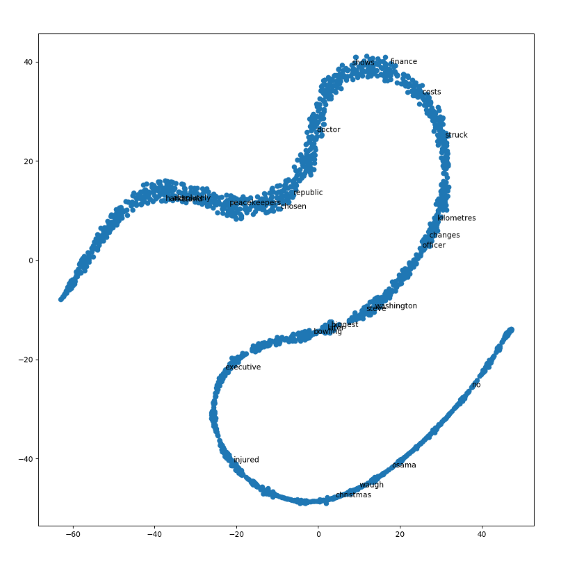
可视化的话语曲面嵌入

通过使用TSNE将单词的维数减少到2维，可以可视化模型制作的单词嵌入。

可视化可用于注意到数据中的语义和句法趋势。

例：

• 语义： words like cat, dog, cow, etc. have a tendency to lie close by

• 句法：words like run, running or cut, cutting lie close together

也可以注意到vKing-vMan = vQueen-vWoman之类的向量关系。

from sklearn.decomposition import IncrementalPCA    # inital reduction
from sklearn.manifold import TSNE                   # final reduction
import numpy as np                                  # array handling

def reduce_dimensions(model):
    num_dimensions = 2  # final num dimensions (2D, 3D, etc)

    vectors = [] # positions in vector space
    labels = [] # keep track of words to label our data again later
    for word in model.wv.vocab:
        vectors.append(model.wv[word])
        labels.append(word)

    # convert both lists into numpy vectors for reduction
    vectors = np.asarray(vectors)
    labels = np.asarray(labels)

    # reduce using t-SNE
    vectors = np.asarray(vectors)
    tsne = TSNE(n_components=num_dimensions, random_state=0)
    vectors = tsne.fit_transform(vectors)

    x_vals = [v[0] for v in vectors]
    y_vals = [v[1] for v in vectors]
    return x_vals, y_vals, labels


x_vals, y_vals, labels = reduce_dimensions(model)

def plot_with_plotly(x_vals, y_vals, labels, plot_in_notebook=True):
    from plotly.offline import init_notebook_mode, iplot, plot
    import plotly.graph_objs as go

    trace = go.Scatter(x=x_vals, y=y_vals, mode='text', text=labels)
    data = [trace]

    if plot_in_notebook:
        init_notebook_mode(connected=True)
        iplot(data, filename='word-embedding-plot')
    else:
        plot(data, filename='word-embedding-plot.html')


def plot_with_matplotlib(x_vals, y_vals, labels):
    import matplotlib.pyplot as plt
    import random

    random.seed(0)

    plt.figure(figsize=(12, 12))
    plt.scatter(x_vals, y_vals)

    #
    # Label randomly subsampled 25 data points
    #
    indices = list(range(len(labels)))
    selected_indices = random.sample(indices, 25)
    for i in selected_indices:
        plt.annotate(labels[i], (x_vals[i], y_vals[i]))

try:
    get_ipython()
except Exception:
    plot_function = plot_with_matplotlib
else:
    plot_function = plot_with_plotly

plot_function(x_vals, y_vals, labels)

 

 

结论

在本教程中，我们学习了如何在自定义数据上训练word2vec模型以及如何对其进行评估。希望您也能在机器学习任务中找到这个受欢迎的工具！