
Understanding q-value and FDR in Differential Expression Analysis
Understanding q-value and FDR in Differential Expression Analysis
Daqian
Introduction to q-value and FDR
In differential gene expression analysis, researchers are often confronted with the challenge of distinguishing true signals — those genes that are genuinely differentially expressed, from the noise — genes that appear to be differentially expressed due to random chance. The p-value is a commonly used statistic to address this issue, but when dealing with thousands of genes, the false discovery rate (FDR) becomes critically important. The q-value is an adjusted p-value that controls for the FDR, and it’s particularly useful in large-scale testing scenarios, such as genomic studies.
The hedenfalk dataset
The hedenfalk dataset includes results from an analysis of gene expression related to BRCA1 and BRCA2 mutations in breast cancer patients. It contains p-values, test statistics, and empirical null statistics for 3170 genes.
Let’s load the dataset and inspect its structure:
library(qvalue)## Warning: package 'qvalue' was built under R version 4.3.1data(hedenfalk)
class(hedenfalk)## [1] "list"names(hedenfalk)## [1] "p" "stat" "stat0"We can extract the p-values and observe the statistics as follows:
pvalues = hedenfalk$p
obs_stats = hedenfalk$stat
null_stats = hedenfalk$stat0

length(obs_stats)
## [1] 3170length(null_stats)## [1] 317000Check the distribution of p-value
Before calculation of the q-value, you are always recommended to check p-values distribution:
hist(hedenfalk$p, nclass = 30)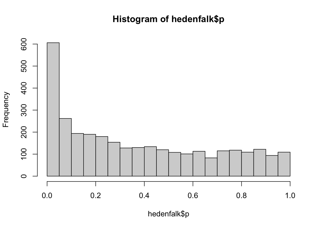
The p-values are relatively flat at the right tail of the histogram. This is an important step in determining whether the true null p-values are distributed according to a Uniform(0,1) distribution.
An important assumption behind the estimation performed in this package is that null p-values follow a Uniform(0,1) distribution, which would result in a p-value histogram where the right tail is fairly flat.
Calculating q-values
Using the qvalue package, we can calculate q-values for each p-value:
qobj = qvalue(p = pvalues)

class(qobj)
## [1] "qvalue"names(qobj)## [1] "call" "pi0" "qvalues" "pvalues" "lfdr"
## [6] "pi0.lambda" "lambda" "pi0.smooth"qvalues = qobj$qvalues
pi0 = qobj$pi0
lfdr = qobj$lfdrA quick summary can be provided by:
summary(qobj)##
## Call:
## qvalue(p = pvalues)
##
## pi0: 0.669926
##
## Cumulative number of significant calls:
##
## <1e-04 <0.001 <0.01 <0.025 <0.05 <0.1 <1
## p-value 15 76 265 424 605 868 3170
## q-value 0 0 1 73 162 319 3170
## local FDR 0 0 3 30 85 167 2241Estimating the Proportion of True Null Hypotheses (\(\pi_0\))
When performing multiple hypothesis tests, one of the key parameters of interest is the proportion of true null hypotheses, often denoted as pi0. This parameter is crucial for understanding the background noise level of non-differential expression in genomic studies.
pi0 is an estimate of the proportion of the total tests for which the null hypothesis is actually true. In other words, it’s an estimate of the percentage of genes in our dataset that are not differentially expressed. Understanding and accurately estimating pi0 is important because it directly affects the calculation of q-values and therefore the FDR.
The qvalue package provides an estimate of pi0 as part of its output: qobj$pi0
The value of \(\pi_0\) can range from 0 to 1: - A \(\pi_0\) close to 1 suggests that most of the genes tested are not differentially expressed, and the majority of the p-values are likely to arise from the null distribution. - A \(\pi_0\) much less than 1 suggests that a substantial proportion of genes are differentially expressed.
The estimate of \(\pi_0\) can be visualized by plotting the p-value distribution and comparing it to the uniform distribution expected under the complete null hypothesis:
hist(qobj)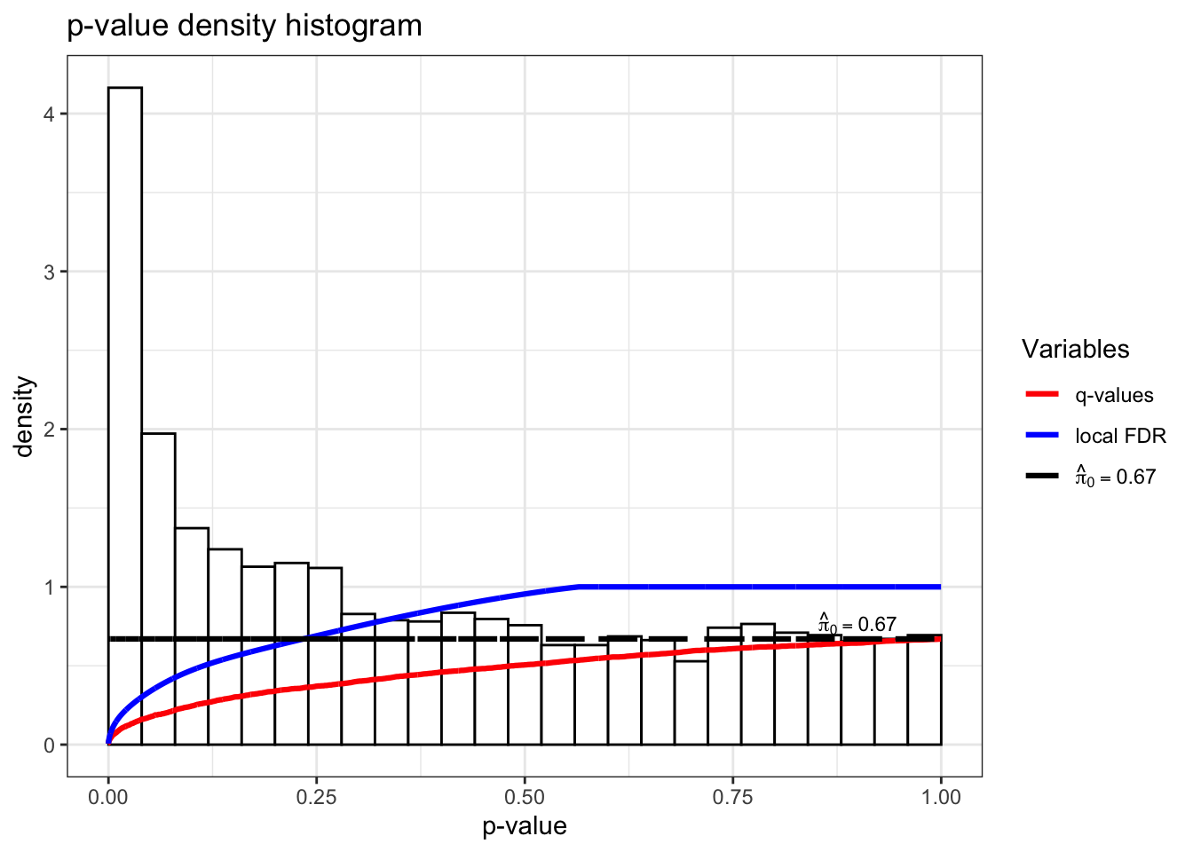
plot(qobj)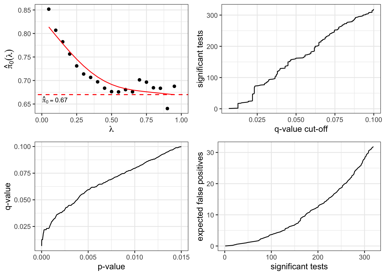
In this plot, the proportion of the p-value distribution that lies above the line \(y = pi0\) is our estimate of the proportion of p-values representing true null hypotheses, i.e., non-differentially expressed genes here. A higher \(\pi_0\) estimate means that we would expect more p-values to be concentrated towards 1, which is characteristic of non-significant results.
Interpreting q-values and FDR
Suppose we have a set of p-values from multiple hypothesis tests and we calculate their corresponding q-values (the case above). The q-values are estimates of the expected proportion of false positives (false discoveries) among all the tests declared significant up to that point.
Let’s say we find that the maximum p-value for which the q-value is less than or equal to 0.05 is 3.81e-03 by running max(pvalues[qobj$qvalues <= 0.05]). This would mean that if we set our significance threshold at a p-value of 3.81e-03, the expected proportion of false discoveries, or the FDR, among the tests deemed significant would not exceed 5%.
So, if we have 1000 genes tested, and 50 of them have p-values less than or equal to 3.81e-03, and we declare these 50 genes as significant, we are operating under an FDR of 5%. In expectation, this would mean that among those 50 significant genes, we expect at most 5% (which would be 2.5 genes in this case, but since we cannot have half a gene, we would interpret this as possibly three of these genes) to be false positives.
In summary, with a maximum p-value of 3.81e-03 corresponding to a q-value threshold of 0.05:
- All genes with p-values ≤
3.81e-03are considered significant. - The expected rate of false discoveries among these significant genes is at most 5%.
Remember that this interpretation is in the context of the entire set of hypothesis tests. Each individual gene with a p-value ≤ 2e-05 doesn’t have a 1% chance of being a false positive; rather, the FDR applies to the group as a whole.
Using a specific FDR level
When we run the qvalue function with an fdr.level = 0.01 argument, we get:
qobj_fdrlevel = qvalue(p = hedenfalk$p, fdr.level = 0.05)
head(qobj_fdrlevel$significant); length(qobj_fdrlevel$significant)
## [1] FALSE FALSE FALSE FALSE FALSE FALSE## [1] 3170This command also yields a logical vector significant, which indicates which genes meet the FDR threshold of 0.01. To get the indices of these genes, we can use:
significant_genes = which(qobj_fdrlevel$significant)
head(significant_genes)
## [1] 10 18 29 35 60 95If we look a step inside we could find the results are equal to the case above (which(qobj$qvalues <= 0.05))
a = which(qobj$qvalues <= 0.05); a## [1] 10 18 29 35 60 95 110 117 130 139 145 151 155 156 254
## [16] 264 267 312 328 329 400 413 434 477 485 488 510 525 542 543
## [31] 571 594 608 627 642 714 723 731 763 786 789 796 821 837 867
## [46] 892 922 930 933 941 942 972 982 994 1038 1040 1057 1060 1063 1072
## [61] 1087 1091 1133 1150 1175 1204 1240 1248 1258 1259 1281 1291 1294 1315 1322
## [76] 1335 1382 1397 1412 1413 1415 1435 1448 1451 1466 1471 1499 1530 1555 1568
## [91] 1573 1586 1594 1612 1730 1731 1779 1797 1815 1823 1838 1885 1932 1962 1981
## [106] 2027 2124 2217 2238 2251 2257 2259 2298 2301 2315 2329 2350 2376 2381 2393
## [121] 2395 2409 2450 2468 2486 2505 2530 2554 2559 2574 2587 2621 2643 2644 2665
## [136] 2671 2682 2684 2703 2734 2754 2818 2841 2852 2880 2898 2922 2924 2929 2945
## [151] 2949 2950 2953 2954 2959 2964 2983 3009 3048 3058 3063 3099b = which(qobj_fdrlevel$significant); b## [1] 10 18 29 35 60 95 110 117 130 139 145 151 155 156 254
## [16] 264 267 312 328 329 400 413 434 477 485 488 510 525 542 543
## [31] 571 594 608 627 642 714 723 731 763 786 789 796 821 837 867
## [46] 892 922 930 933 941 942 972 982 994 1038 1040 1057 1060 1063 1072
## [61] 1087 1091 1133 1150 1175 1204 1240 1248 1258 1259 1281 1291 1294 1315 1322
## [76] 1335 1382 1397 1412 1413 1415 1435 1448 1451 1466 1471 1499 1530 1555 1568
## [91] 1573 1586 1594 1612 1730 1731 1779 1797 1815 1823 1838 1885 1932 1962 1981
## [106] 2027 2124 2217 2238 2251 2257 2259 2298 2301 2315 2329 2350 2376 2381 2393
## [121] 2395 2409 2450 2468 2486 2505 2530 2554 2559 2574 2587 2621 2643 2644 2665
## [136] 2671 2682 2684 2703 2734 2754 2818 2841 2852 2880 2898 2922 2924 2929 2945
## [151] 2949 2950 2953 2954 2959 2964 2983 3009 3048 3058 3063 3099a == b## [1] TRUE TRUE TRUE TRUE TRUE TRUE TRUE TRUE TRUE TRUE TRUE TRUE TRUE TRUE TRUE
## [16] TRUE TRUE TRUE TRUE TRUE TRUE TRUE TRUE TRUE TRUE TRUE TRUE TRUE TRUE TRUE
## [31] TRUE TRUE TRUE TRUE TRUE TRUE TRUE TRUE TRUE TRUE TRUE TRUE TRUE TRUE TRUE
## [46] TRUE TRUE TRUE TRUE TRUE TRUE TRUE TRUE TRUE TRUE TRUE TRUE TRUE TRUE TRUE
## [61] TRUE TRUE TRUE TRUE TRUE TRUE TRUE TRUE TRUE TRUE TRUE TRUE TRUE TRUE TRUE
## [76] TRUE TRUE TRUE TRUE TRUE TRUE TRUE TRUE TRUE TRUE TRUE TRUE TRUE TRUE TRUE
## [91] TRUE TRUE TRUE TRUE TRUE TRUE TRUE TRUE TRUE TRUE TRUE TRUE TRUE TRUE TRUE
## [106] TRUE TRUE TRUE TRUE TRUE TRUE TRUE TRUE TRUE TRUE TRUE TRUE TRUE TRUE TRUE
## [121] TRUE TRUE TRUE TRUE TRUE TRUE TRUE TRUE TRUE TRUE TRUE TRUE TRUE TRUE TRUE
## [136] TRUE TRUE TRUE TRUE TRUE TRUE TRUE TRUE TRUE TRUE TRUE TRUE TRUE TRUE TRUE
## [151] TRUE TRUE TRUE TRUE TRUE TRUE TRUE TRUE TRUE TRUE TRUE TRUEConclusion
The q-value is a powerful tool for researchers performing large-scale hypothesis testing, as it provides a means to control the false discovery rate. By utilizing the qvalue package in R, we can confidently identify genes that are truly differentially expressed, while minimizing the rate of false positives. This is crucial in fields like genomics, where the sheer number of simultaneous tests can lead to a high number of false discoveries if not properly controlled.

 浙公网安备 33010602011771号