机器学习(4)之Logistic回归

2014-09-11 23:17 追风的蓝宝阅读(1289) 评论(0) 编辑收藏举报

机器学习(4)之Logistic回归

1. 算法推导　

与之前学过的梯度下降等不同，Logistic回归是一类分类问题，而前者是回归问题。回归问题中，尝试预测的变量y是连续的变量，而在分类问题中，y是一组离散的，比如y只能取{0,1}。

　　假设一组样本为这样如图所示，如果需要用线性回归来拟合这些样本，匹配效果会很不好。对于这种y值只有{0,1}这种情况的，可以使用分类方法进行。

假设，且使得

其中定义Logistic函数(又名sigmoid函数)：

下图是Logistic函数g(z)的分布曲线，当z大时候g(z)趋向1，当z小的时候g(z)趋向0，z=0时候g(z)=0.5,因此将g(z)控制在{0,1}之间。其他的g(z)函数只要是在{0,1}之间就同样可以，但是后续的章节会讲到，现在所使用的sigmoid函数是最常用的

假设给定x以为参数的y=1和y=0的概率：

可以简写成：

假设m个训练样本都是独立的，那么θ的似然函数可以写成：

对L(θ)求解对数最大似然值：

为了使似然性最大化，类似于线性回归使用梯度下降的方法，求对数似然性对的偏导，即：

注意：之前的梯度下降算法的公式为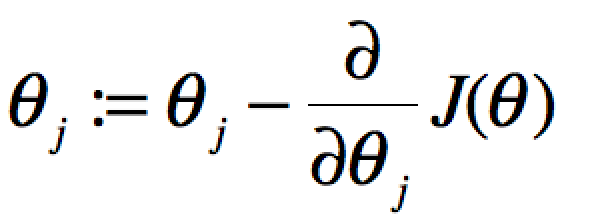。这是是梯度上升，Θ:=Θ的含义就是前后两次迭代(或者说前后两个样本)的变化值为l(Θ)的导数。

则

即类似上节课的随机梯度上升算法，形式上和线性回归是相同的，只是符号相反，为logistic函数，但实质上和线性回归是不同的学习算法。

2. 改进的Logistic回归算法

评价一个优化算法的优劣主要是看它是否收敛，也就是说参数是否达到稳定值，是否还会不断的变化？收敛速度是否快？

上图展示了随机梯度下降算法在200次迭代中（请先看第三和第四节再回来看这里。我们的数据库有100个二维样本，每个样本都对系数调整一次，所以共有200*100=20000次调整）三个回归系数的变化过程。其中系数X2经过50次迭代就达到了稳定值。但系数X1和X0到100次迭代后稳定。而且可恨的是系数X1和X2还在很调皮的周期波动，迭代次数很大了，心还停不下来。产生这个现象的原因是存在一些无法正确分类的样本点，也就是我们的数据集并非线性可分，但我们的logistic regression是线性分类模型，对非线性可分情况无能为力。然而我们的优化程序并没能意识到这些不正常的样本点，还一视同仁的对待，调整系数去减少对这些样本的分类误差，从而导致了在每次迭代时引发系数的剧烈改变。对我们来说，我们期待算法能避免来回波动，从而快速稳定和收敛到某个值。

对随机梯度下降算法，我们做两处改进来避免上述的波动问题：

1）在每次迭代时，调整更新步长alpha的值。随着迭代的进行，alpha越来越小，这会缓解系数的高频波动（也就是每次迭代系数改变得太大，跳的跨度太大）。当然了，为了避免alpha随着迭代不断减小到接近于0（这时候，系数几乎没有调整，那么迭代也没有意义了），我们约束alpha一定大于一个稍微大点的常数项，具体见代码。

2）每次迭代，改变样本的优化顺序。也就是随机选择样本来更新回归系数。这样做可以减少周期性的波动，因为样本顺序的改变，使得每次迭代不再形成周期性。

改进的随机梯度下降算法的伪代码如下：

################################################

初始化回归系数为1

重复下面步骤直到收敛{

对随机遍历的数据集中的每个样本

随着迭代的逐渐进行，减小alpha的值

计算该样本的梯度

使用alpha x gradient来更新回归系数

}

返回回归系数值

################################################

比较原始的随机梯度下降和改进后的梯度下降，可以看到两点不同：

1）系数不再出现周期性波动。2）系数可以很快的稳定下来，也就是快速收敛。这里只迭代了20次就收敛了。而上面的随机梯度下降需要迭代200次才能稳定。

3. python实现

 1 # coding=utf-8
 2 #!/usr/bin/python
 3 #Filename:LogisticRegression.py
 4 '''
 5 Created on 2014年9月13日
 6  
 7 @author: Ryan C. F.
 8 
 9 '''
10 
11 from numpy import *
12 import matplotlib.pyplot as plt
13 import time
14 
15 def sigmoid(inX):  
16     ''' 
17     simoid  函数
18     '''
19     return 1.0 / (1 + exp(-inX))
20 
21 def trainLogRegres(train_x, train_y, opts):  
22     '''
23     train a logistic regression model using some optional optimize algorithm  
24     input: train_x is a mat datatype, each row stands for one sample  
25     train_y is mat datatype too, each row is the corresponding label  
26     opts is optimize option include step and maximum number of iterations  
27     '''
28     # calculate training time  
29     startTime = time.time()  
30   
31     numSamples, numFeatures = shape(train_x)  
32     alpha = opts['alpha']; maxIter = opts['maxIter']  
33     weights = ones((numFeatures, 1))  
34   
35     # optimize through gradient ascent algorilthm  
36     for k in range(maxIter):  
37         if opts['optimizeType'] == 'gradAscent': # gradient ascent algorilthm  
38             output = sigmoid(train_x * weights)  
39             error = train_y - output  
40             weights = weights + alpha * train_x.transpose() * error  
41         elif opts['optimizeType'] == 'stocGradAscent': # stochastic gradient ascent  
42             for i in range(numSamples):  
43                 output = sigmoid(train_x[i, :] * weights)  
44                 error = train_y[i, 0] - output  
45                 weights = weights + alpha * train_x[i, :].transpose() * error  
46         elif opts['optimizeType'] == 'smoothStocGradAscent': # smooth stochastic gradient ascent  
47             # randomly select samples to optimize for reducing cycle fluctuations   
48             dataIndex = range(numSamples)  
49             for i in range(numSamples):  
50                 alpha = 4.0 / (1.0 + k + i) + 0.01  
51                 randIndex = int(random.uniform(0, len(dataIndex)))  
52                 output = sigmoid(train_x[randIndex, :] * weights)  
53                 error = train_y[randIndex, 0] - output  
54                 weights = weights + alpha * train_x[randIndex, :].transpose() * error  
55                 del(dataIndex[randIndex]) # during one interation, delete the optimized sample  
56         else:  
57             raise NameError('Not support optimize method type!')  
58       
59   
60     print 'Congratulations, training complete! Took %fs!' % (time.time() - startTime)  
61     return weights  
62 
63 # test your trained Logistic Regression model given test set  
64 def testLogRegres(weights, test_x, test_y):  
65     numSamples, numFeatures = shape(test_x)  
66     matchCount = 0  
67     for i in xrange(numSamples):  
68         predict = sigmoid(test_x[i, :] * weights)[0, 0] > 0.5  
69         if predict == bool(test_y[i, 0]):  
70             matchCount += 1  
71     accuracy = float(matchCount) / numSamples  
72     return accuracy  
73   
74   
75 # show your trained logistic regression model only available with 2-D data  
76 def showLogRegres(weights, train_x, train_y):  
77     # notice: train_x and train_y is mat datatype  
78     numSamples, numFeatures = shape(train_x)  
79     if numFeatures != 3:  
80         print "Sorry! I can not draw because the dimension of your data is not 2!"  
81         return 1  
82   
83     # draw all samples  
84     for i in xrange(numSamples):  
85         if int(train_y[i, 0]) == 0:  
86             plt.plot(train_x[i, 1], train_x[i, 2], 'or')  
87         elif int(train_y[i, 0]) == 1:  
88             plt.plot(train_x[i, 1], train_x[i, 2], 'ob')  
89   
90     # draw the classify line  
91     min_x = min(train_x[:, 1])[0, 0]  
92     max_x = max(train_x[:, 1])[0, 0]  
93     weights = weights.getA()  # convert mat to array  
94     y_min_x = float(-weights[0] - weights[1] * min_x) / weights[2]  
95     y_max_x = float(-weights[0] - weights[1] * max_x) / weights[2]  
96     plt.plot([min_x, max_x], [y_min_x, y_max_x], '-g')  
97     plt.xlabel('X1'); plt.ylabel('X2')  
98     plt.show()

 1 # coding=utf-8
 2 #!/usr/bin/python
 3 #Filename:testLogisticRegression.py
 4 '''
 5 Created on 2014年9月13日
 6  
 7 @author: Ryan C. F.
 8 
 9 '''
10 
11 from numpy import *  
12 import matplotlib.pyplot as plt  
13 import time  
14 from LogisticRegression import *
15 
16 def loadData():  
17     train_x = []  
18     train_y = []  
19     fileIn = open('/Users/rcf/workspace/java/workspace/MachineLinearing/src/supervisedLearning/trains.txt')  
20     for line in fileIn.readlines():  
21         lineArr = line.strip().split()  
22         train_x.append([1.0, float(lineArr[0]), float(lineArr[1])])  
23         train_y.append(float(lineArr[2]))  
24     return mat(train_x), mat(train_y).transpose()  
25   
26   
27 ## step 1: load data  
28 print "step 1: load data..."
29 train_x, train_y = loadData() 
30 test_x = train_x; test_y = train_y  
31 print train_x
32 print train_y
33 ## step 2: training...  
34 print "step 2: training..."  
35 opts = {'alpha': 0.001, 'maxIter': 100, 'optimizeType': 'smoothStocGradAscent'}
36 optimalWeights = trainLogRegres(train_x, train_y, opts)  
37   
38 ## step 3: testing  
39 print "step 3: testing..."  
40 accuracy = testLogRegres(optimalWeights, test_x, test_y)  
41   
42 ## step 4: show the result  
43 print "step 4: show the result..."    
44 print 'The classify accuracy is: %.3f%%' % (accuracy * 100)  
45 showLogRegres(optimalWeights, train_x, train_y)

  1 -0.017612    14.053064    0
  2 -1.395634    4.662541    1
  3 -0.752157    6.538620    0
  4 -1.322371    7.152853    0
  5 0.423363    11.054677    0
  6 0.406704    7.067335    1
  7 0.667394    12.741452    0
  8 -2.460150    6.866805    1
  9 0.569411    9.548755    0
 10 -0.026632    10.427743    0
 11 0.850433    6.920334    1
 12 1.347183    13.175500    0
 13 1.176813    3.167020    1
 14 -1.781871    9.097953    0
 15 -0.566606    5.749003    1
 16 0.931635    1.589505    1
 17 -0.024205    6.151823    1
 18 -0.036453    2.690988    1
 19 -0.196949    0.444165    1
 20 1.014459    5.754399    1
 21 1.985298    3.230619    1
 22 -1.693453    -0.557540    1
 23 -0.576525    11.778922    0
 24 -0.346811    -1.678730    1
 25 -2.124484    2.672471    1
 26 1.217916    9.597015    0
 27 -0.733928    9.098687    0
 28 -3.642001    -1.618087    1
 29 0.315985    3.523953    1
 30 1.416614    9.619232    0
 31 -0.386323    3.989286    1
 32 0.556921    8.294984    1
 33 1.224863    11.587360    0
 34 -1.347803    -2.406051    1
 35 1.196604    4.951851    1
 36 0.275221    9.543647    0
 37 0.470575    9.332488    0
 38 -1.889567    9.542662    0
 39 -1.527893    12.150579    0
 40 -1.185247    11.309318    0
 41 -0.445678    3.297303    1
 42 1.042222    6.105155    1
 43 -0.618787    10.320986    0
 44 1.152083    0.548467    1
 45 0.828534    2.676045    1
 46 -1.237728    10.549033    0
 47 -0.683565    -2.166125    1
 48 0.229456    5.921938    1
 49 -0.959885    11.555336    0
 50 0.492911    10.993324    0
 51 0.184992    8.721488    0
 52 -0.355715    10.325976    0
 53 -0.397822    8.058397    0
 54 0.824839    13.730343    0
 55 1.507278    5.027866    1
 56 0.099671    6.835839    1
 57 -0.344008    10.717485    0
 58 1.785928    7.718645    1
 59 -0.918801    11.560217    0
 60 -0.364009    4.747300    1
 61 -0.841722    4.119083    1
 62 0.490426    1.960539    1
 63 -0.007194    9.075792    0
 64 0.356107    12.447863    0
 65 0.342578    12.281162    0
 66 -0.810823    -1.466018    1
 67 2.530777    6.476801    1
 68 1.296683    11.607559    0
 69 0.475487    12.040035    0
 70 -0.783277    11.009725    0
 71 0.074798    11.023650    0
 72 -1.337472    0.468339    1
 73 -0.102781    13.763651    0
 74 -0.147324    2.874846    1
 75 0.518389    9.887035    0
 76 1.015399    7.571882    0
 77 -1.658086    -0.027255    1
 78 1.319944    2.171228    1
 79 2.056216    5.019981    1
 80 -0.851633    4.375691    1
 81 -1.510047    6.061992    0
 82 -1.076637    -3.181888    1
 83 1.821096    10.283990    0
 84 3.010150    8.401766    1
 85 -1.099458    1.688274    1
 86 -0.834872    -1.733869    1
 87 -0.846637    3.849075    1
 88 1.400102    12.628781    0
 89 1.752842    5.468166    1
 90 0.078557    0.059736    1
 91 0.089392    -0.715300    1
 92 1.825662    12.693808    0
 93 0.197445    9.744638    0
 94 0.126117    0.922311    1
 95 -0.679797    1.220530    1
 96 0.677983    2.556666    1
 97 0.761349    10.693862    0
 98 -2.168791    0.143632    1
 99 1.388610    9.341997    0
100 0.317029    14.739025    0