监督学习
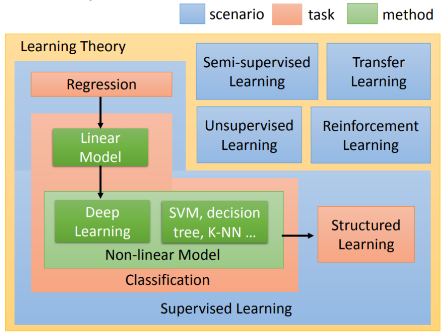
1. 监督学习和无监督学习
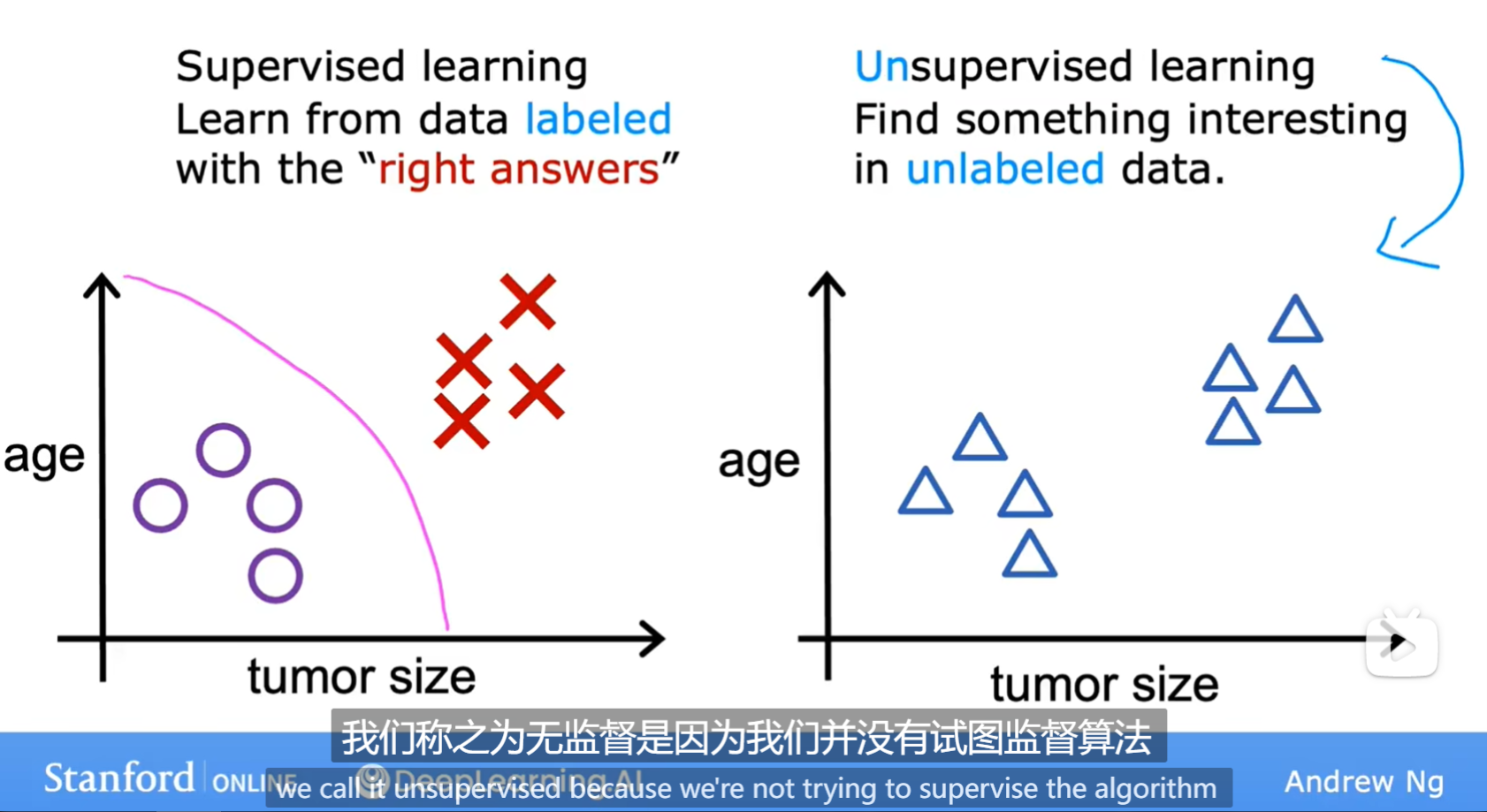
- 监督学习有规定的输入输出,无监督学习没有
监督学习的两种主要类型:回归和分类
举例无监督学习:
- 聚类(clustering algorithm):例如将搜索界面将相关的新闻关联在一起、找到DNA有共性的分组、分析主要用户需求
- 异常检测(anomaly detection):检测异常
- 降维(dimensionality reduction):将大数据组降成小数据组,同时丢失尽量少的信息
2. 线性回归(linear regression)
\[y = wx + b
\]
使用\((x^{(i)} , y^{(i)})\)表示数据中第i对值
Numpy数组有一个 .shape 参数。x_train.shape 返回一个 python 元组,每个维度都有一个条目。x_train.shape[0] 是数组的长度和示例数
import numpy as np
import matplotlib.pyplot as plt
x_train = np.array([1.0, 2.0])
y_train = np.array([300.0, 500.0])
print(f"x_train.shape: {x_train.shape}")
m = x_train.shape[0]
print(f"Number of training examples is: {m}")
输出结果为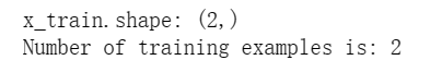
也可以使用len,即m = len(x_train),输出结果仍为2
# Plot the data points
plt.scatter(x_train, y_train, marker='x', c='r')
# Set the title
plt.title("Housing Prices")
# Set the y-axis label
plt.ylabel('Price (in 1000s of dollars)')
# Set the x-axis label
plt.xlabel('Size (1000 sqft)')
plt.show()
绘制如图: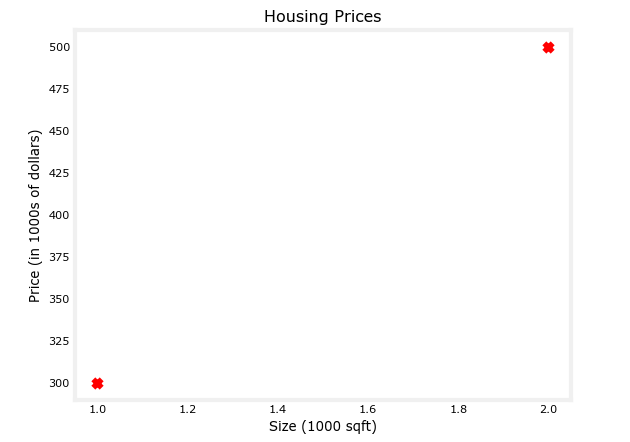
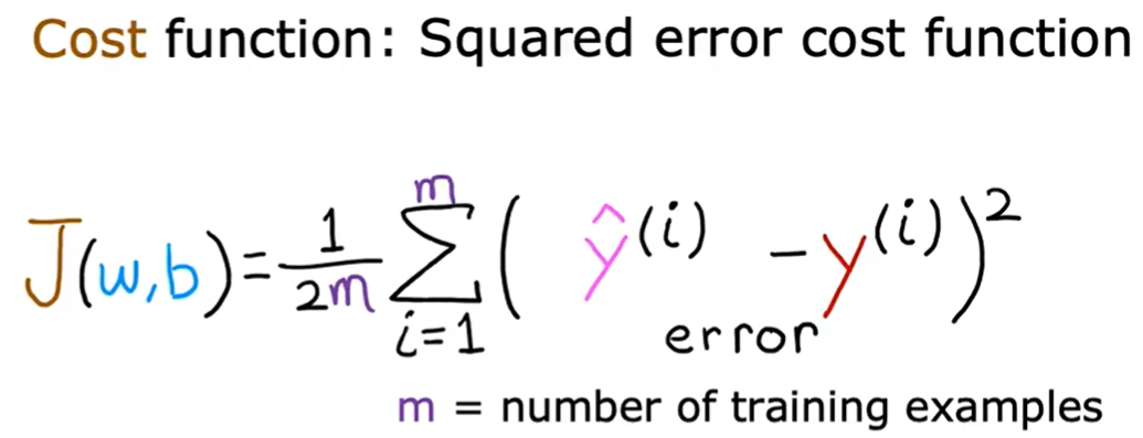
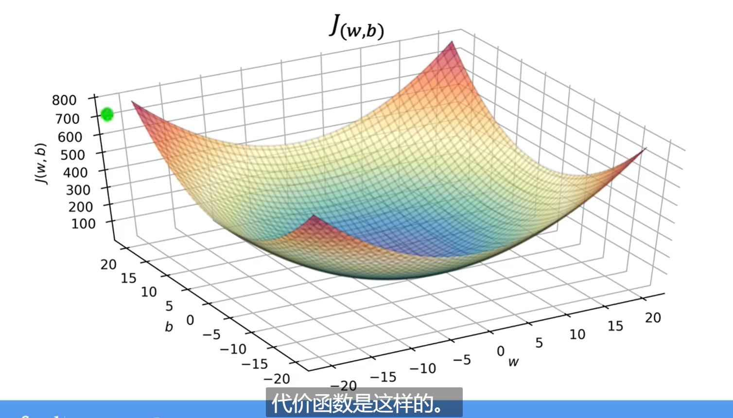
3. 代价函数
代价函数是评价回归模型的一个指标,有助于优化模型
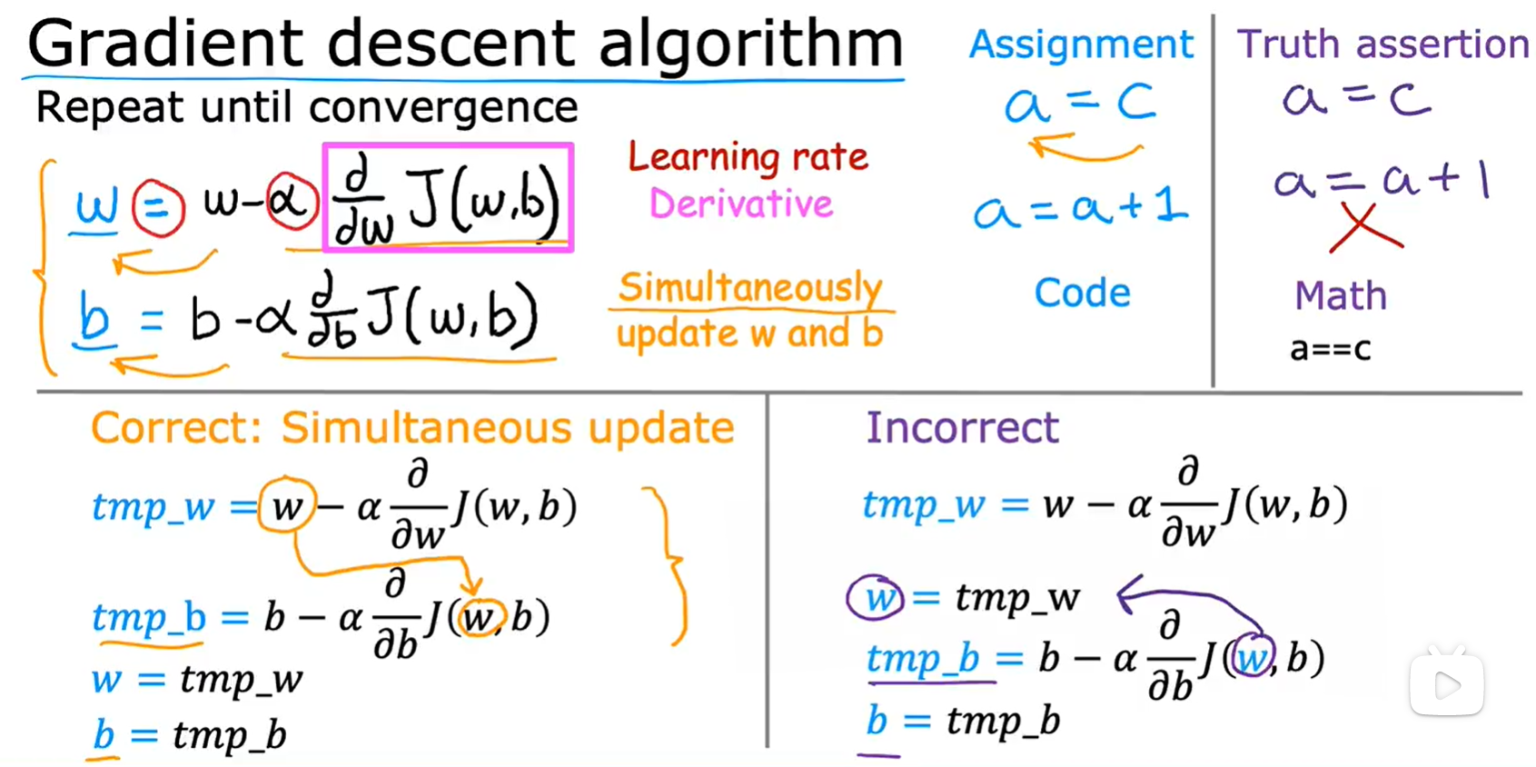
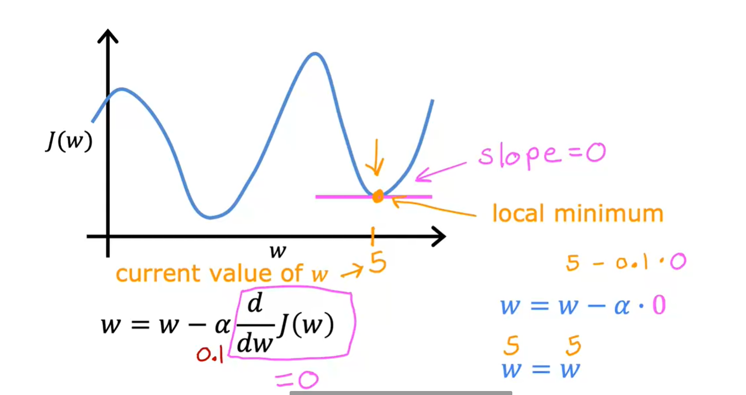
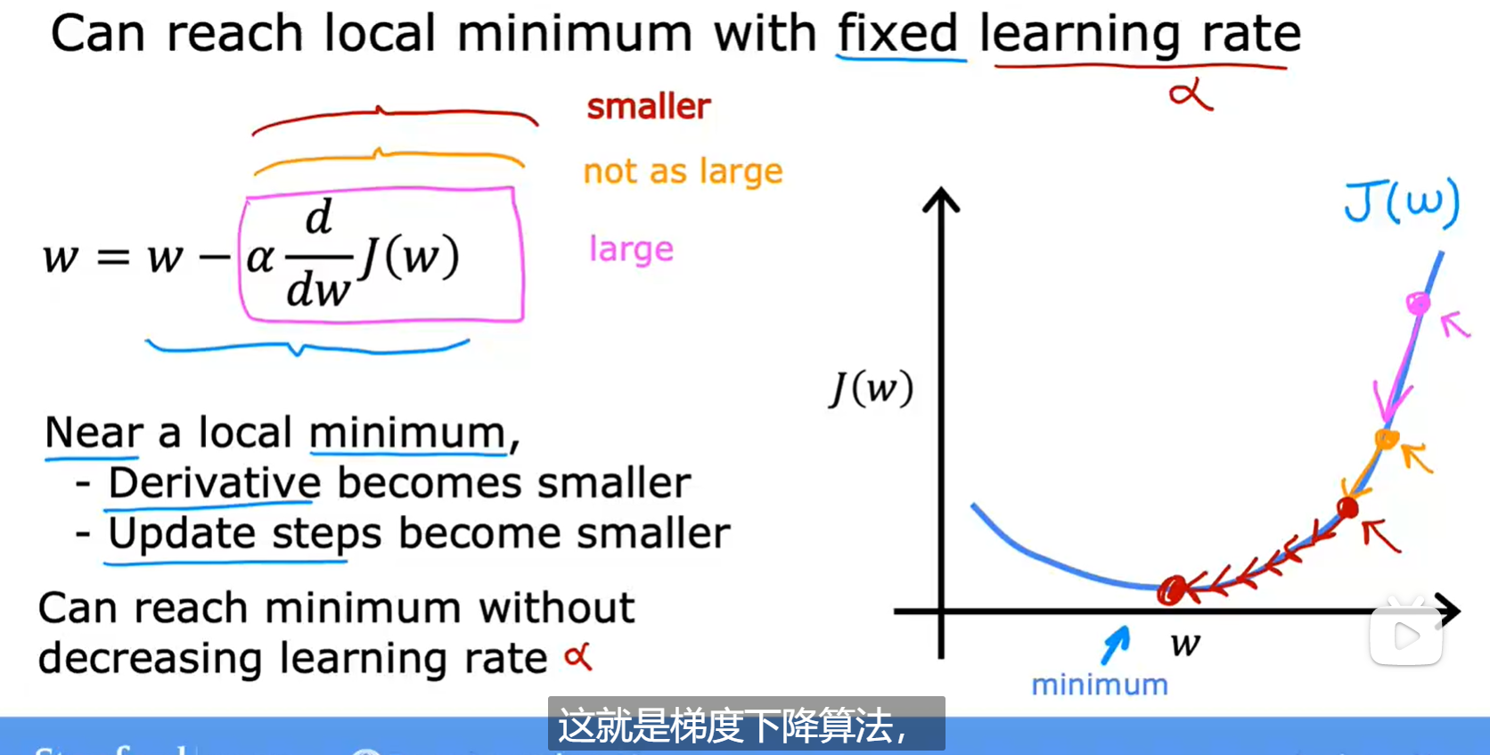
4. 梯度下降
梯度下降参考博客:梯度下降(Gradient Descent)小结
梯度下降法(Grandient descent)
f函数的计算如下:
# Function to calculate the cost:算出代价
def compute_cost(x, y, w, b):

    m = x.shape[0] //m是x的行数,array.shape[0]是行数,array.shape[1]是列数
    cost = 0

    for i in range(m):
        f_wb = w * x[i] + b
        cost = cost + (f_wb - y[i])**2
    total_cost = 1 / (2 * m) * cost

    return total_cost
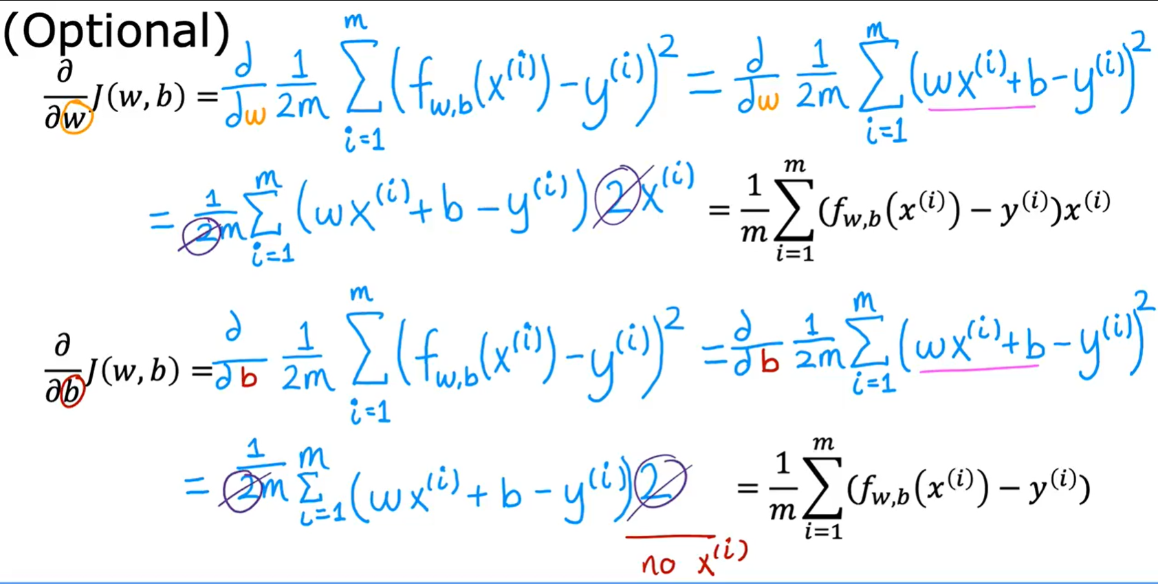
求偏导:
def compute_gradient(x, y, w, b):
    """
    Computes the gradient for linear regression
    Args:
      x (ndarray (m,)): Data, m examples
      y (ndarray (m,)): target values
      w,b (scalar)    : model parameters
    Returns
      dj_dw (scalar): The gradient of the cost w.r.t. the parameters w
      dj_db (scalar): The gradient of the cost w.r.t. the parameter b
     """

    # Number of training examples
    m = x.shape[0]
    dj_dw = 0
    dj_db = 0

    for i in range(m):
        f_wb = w * x[i] + b
        dj_dw_i = (f_wb - y[i]) * x[i]
        dj_db_i = f_wb - y[i]
        dj_db += dj_db_i
        dj_dw += dj_dw_i
    dj_dw = dj_dw / m
    dj_db = dj_db / m

    return dj_dw, dj_db
梯度下降函数:
def gradient_descent(x, y, w_in, b_in, cost_function, gradient_function, alpha, num_iters):
    """
    Performs batch gradient descent to learn theta. Updates theta by taking
    num_iters gradient steps with learning rate alpha

    Args:
      x :    (ndarray): Shape (m,)
      y :    (ndarray): Shape (m,)
      w_in, b_in : (scalar) Initial values of parameters of the model
      cost_function: function to compute cost
      gradient_function: function to compute the gradient
      alpha : (float) Learning rate
      num_iters : (int) number of iterations to run gradient descent
    Returns
      w : (ndarray): Shape (1,) Updated values of parameters of the model after
          running gradient descent
      b : (scalar)                Updated value of parameter of the model after
          running gradient descent
    """

    # number of training examples
    m = len(x)

    # An array to store cost J and w's at each iteration — primarily for graphing later
    J_history = []
    w_history = []
    w = copy.deepcopy(w_in)  #avoid modifying global w within function
    b = b_in

    for i in range(num_iters):

        # Calculate the gradient and update the parameters
        dj_dw, dj_db = gradient_function(x, y, w, b )

        # Update Parameters using w, b, alpha and gradient
        w = w - alpha * dj_dw
        b = b - alpha * dj_db

        # Save cost J at each iteration
        if i<100000:      # prevent resource exhaustion
            cost =  cost_function(x, y, w, b)
            J_history.append(cost)

        # Print cost every at intervals 10 times or as many iterations if < 10
        if i% math.ceil(num_iters/10) == 0:
            w_history.append(w)
            print(f"Iteration {i:4}: Cost {float(J_history[-1]):8.2f}   ")

    return w, b, J_history, w_history #return w and J,w history for graphing
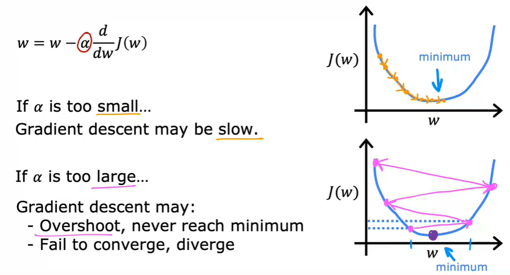
4.1 学习率
学习率太小可能迭代过慢
学习率太大可能不收敛,甚至发散

 浙公网安备 33010602011771号