
cs294-ai-sys2022 lectures6 reading
1. On Large-Batch Training for Deep Learning: Generalization Gap and Sharp Minima(Optional 2017 Northwestern University)
- 动机
- SGD and its variants理论属性:
-
convergence to minimizers of strongly-convex functions and to stationary points for non-convex functions
-
saddle-point avoidance
- robustness to input data
-
- SGD问题
-
owing to the sequential nature of the iteration(数据并行等方式可缓解吧?) and small batch sizes, there is limited avenue for parallelization
-
- SGD and its variants理论属性:
- 工作
-
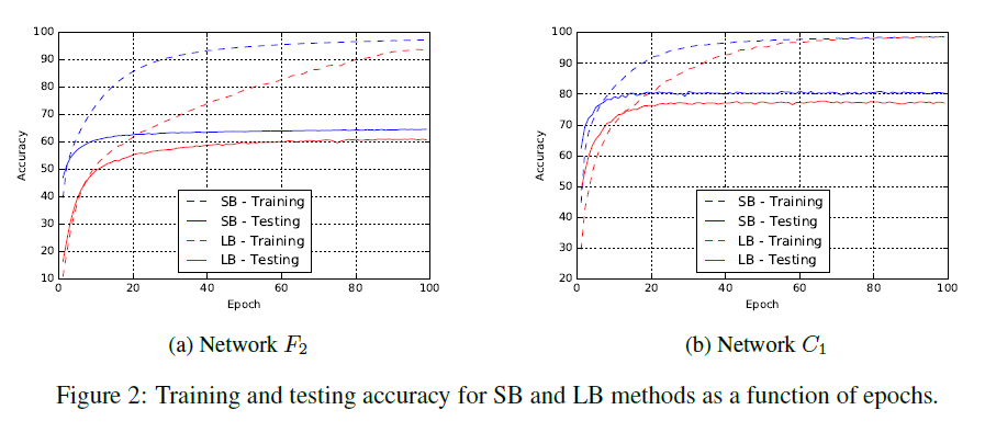
We observe that the generalization gap is correlated with a marked sharpness of the minimizersobtained by large-batch methods. This motivates efforts at remedying the generalization problem
-
- DRAWBACKS OF LARGE-BATCH METHODS
- OUR MAIN OBSERVATION
-
LB(Large-Batch) methods lack the explorative properties of SB(Small-Batch) methods and tend to zoom-in on the minimizer closest to the initial point
-
SB and LB methods converge to qualitatively different minimizers with differing generalization properties
-
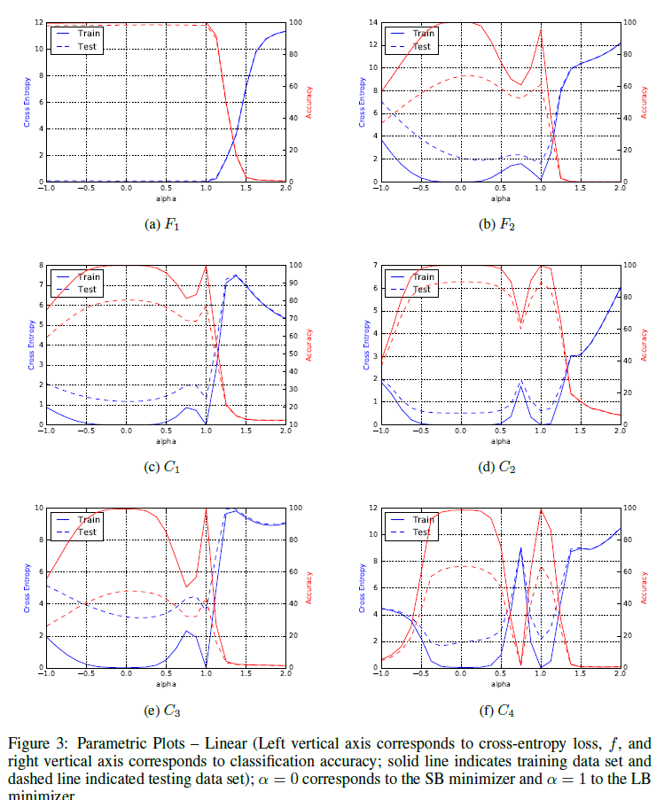
The lack of generalization ability is due to the fact that large-batch methods tend to converge to sharp minimizers of the training function. These minimizers are characterized by a significant number of large positive eigenvalues(特征值) in 损失函数二阶导数矩阵, and tend to generalize less well. In contrast, small-batch methods converge to flat minimizers characterized by having numerous small eigenvalues of 损失函数二阶导数矩阵. We have observed that the loss function landscape of deep neural networks is such that large-batch methods are attracted to regions with sharp minimizers and that, unlike small-batch methods, are unable to escape basins of attraction of these minimizers.
-
- NUMERICAL EXPERIMENTS
-
We emphasize that the generalization gap is not due to over-fitting or over-training as commonly observed in statistics. Early-stopping heuristics aimed at preventing models from over-fitting would not help reduce the generalization gap.
-
- OUR MAIN OBSERVATION

-
-
- we describe approaches to attempt to remedy this generalization problem of LB methods. These approaches include data augmentation, conservative training and adversarial training. Our preliminary findings show that these approaches help reduce the generalization gap but still lead to relatively sharp minimizers and as such, do not completely remedy the problem
-
We conclude this section by noting that the sharp minimizers identified in our experiments do not resemble a cone(不是圆锥形), i.e., the function does not increase rapidly along all (or even most) directions. By sampling the loss function in a neighborhood of LB solutions, we observe that it rises steeply only along a small dimensional subspace (e.g. 5% of the whole space); on most other directions, the function is relatively
-
- SUCCESS OF SMALL-BATCH METHODS
-
Let us now consider the behavior of SB methods, which use noisy gradients in the step computation. From the results reported in the previous section, it appears that noise in the gradient pushes the iterates out of the basin of attraction of sharp minimizers and encourages movement towards a flatter minimizer where noise will not cause exit from that basin.
-
It has been speculated that LB methods tend to be attracted to minimizers close to the starting pointx0, whereas SB methods move away and locate minimizers that are farther away
-
As the loss function reduces, the sharpness of the iterates corresponding to the LB method rapidly increases, whereas for the SB method the sharpness stays relatively constant initially and then reduces, suggesting an exploration phase followed by convergence to a flat minimizer.
-
-
use of dynamic sampling where the batch size is increased gradually as the iteration progresses . The potential viability of this approach is suggested by our warm-starting experiments wherein high testing accuracy is achieved using a large-batch method that is warm-start with a small-batch method.
2. Large Batch Optimization for Deep Learning: Training BERT in 76 minutes(Optional 2020 Google)
- 动机
-
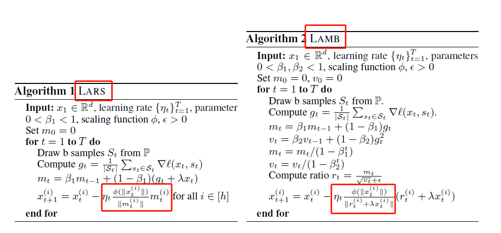
There has been recent surge in interest in using large batch stochastic optimization methods to tackle this issue. The most prominent algorithm in this line of research is LARS, which by employing layerwise adaptive learning rates trains RESNET on ImageNet in a few minutes. However, LARS performs poorly for attention models like BERT, indicating that its performance gains are not consistent across tasks
- linear scaling in large batch synchronous SGD
-
linear scaling of learning rate is harmful during the initial phase; thus, a hand-tuned warmup strategy of slowly increasing the learning rate needs to be used initially
- linear scaling of learning rate can be detrimental beyond a certain batch size
-
empirical study (Shallue et al., 2018) shows that learning rate scaling heuristics with the batch size do not hold across all problems or across all batch sizes
-
-
- 工作
-
Inspired by LARS, we investigate a general adaptation strategy specially catered to large batch learning and provide intuition for the strategy
-
we develop a new optimization algorithm (LAMB) for achieving adaptivity of learning rate in SGD
-
- ALGORITHMS
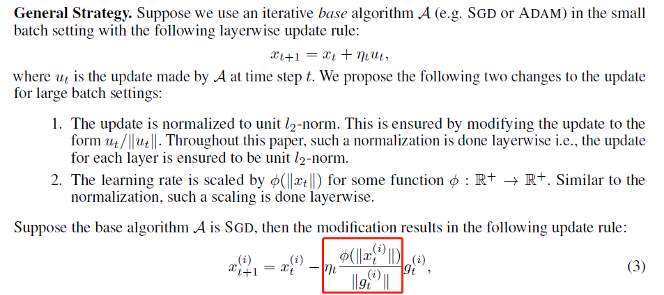
- General Strategy
-
Normalization of this form essentially ignores the size of the gradient and is particularly useful in large batch settings where the direction of the gradient is largely preserved.
-
The scaling term involving ensures that the norm of the update is of the same order as that of the parameter
![]()
-
- LARS ALGORITHM and LAMB ALGORITHM
-
we maintain the same training procedure as the baseline except for changing the training optimizer to LAMB. We run with the same number of epochs as the baseline but with batch size scaled from 512 to 32K. The choice of 32K batch size (with sequence length 512) is mainly
due to memory limits of TPU Pod -
we use the Mixed-Batch Training procedure with LAMB. Recall that BERT training involves two stages: the first 9/10 of the total epochs use a sequence length of 128, while the last 1/10 of the total epochs use a sequence length of 512. we can potentially use a larger batch size for the first stage because of a shorter sequence length, we restrict the batch size to 65536 for this stage
-
![]()
-
- General Strategy
3. Measuring the Effects of Data Parallelism on Neural Network Training(Require 2020, Google)
- 动机
-
For many important problems, the best models are still improving at the end of training because practitioners cannot afford to wait until the performance saturates(现实情况,所以目标不是达到最优,而是如何在成本有限的情况下得到最好的模型)
-
Practitioners are primarily concerned with out-of-sample error and the cost they pay to achieve that error. Cost can be measured in a variety of ways, including training time and hardware costs. Training time can be decomposed into number of steps multiplied by average time per step, and hardware cost into number of steps multiplied by average hardware cost per step. The per-step time and hardware costs depend on the practitioner's hardware, but the number of training steps is hardware-agnostic and can be used to compute the total costs for any hardware given its per-step costs. Furthermore, in an idealized dataparallel system where the communication overhead between processors is negligible
-
- 工作
-
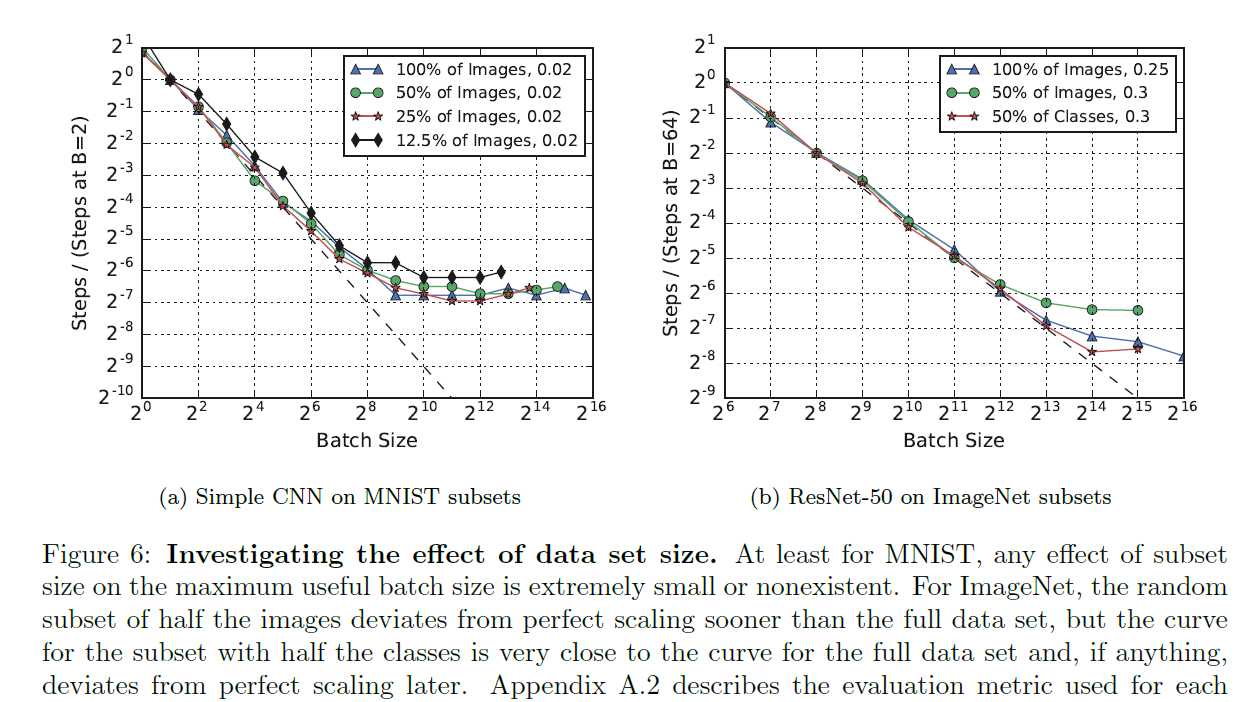
We show that the maximum useful batch size varies significantly between workloads and depends on properties of the model, training algorithm, and data set
-
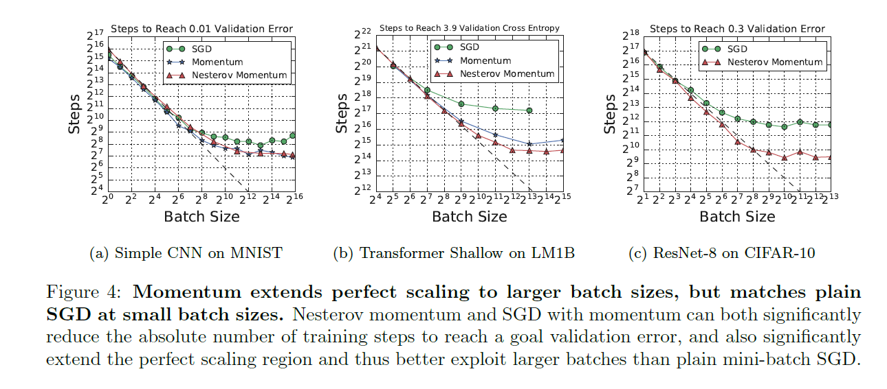
SGD with momentum (as well as Nesterov momentum) can make use of much larger batch sizes than plain SGD
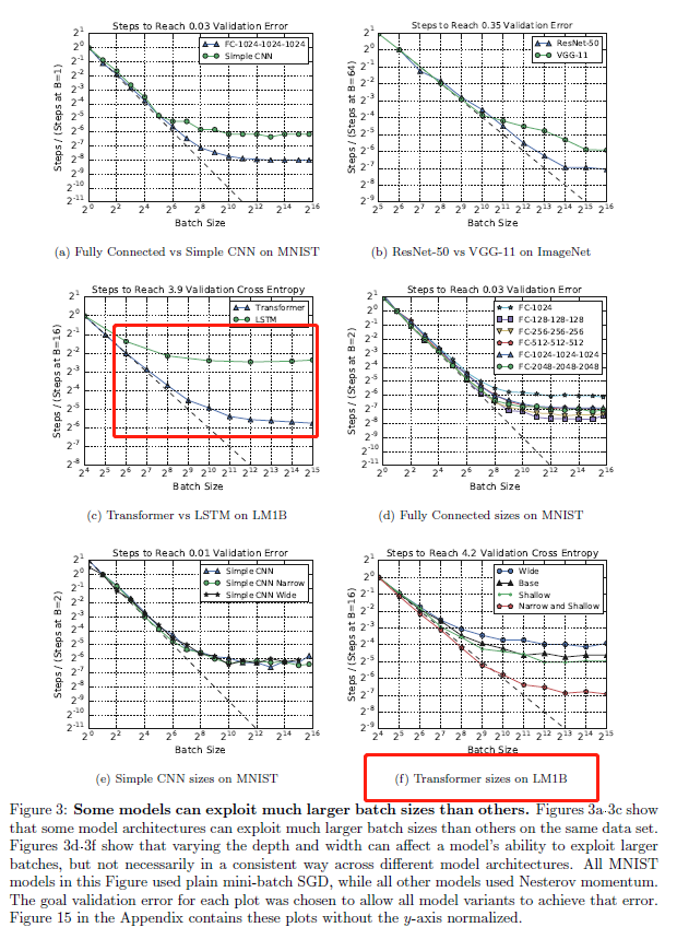
- Some models allow training to scale to much larger batch sizes than others
-
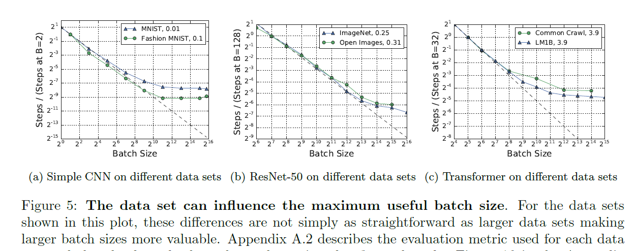
The effect of the data set on the maximum useful batch size tends to be smaller than the effects of the model and training algorithm
-
-
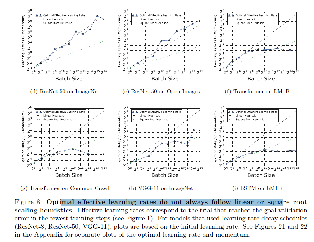
popular learning rate heuristics, such as linearly scaling the learning rate with the batch size do not hold across all problems or across all batch sizes.
-
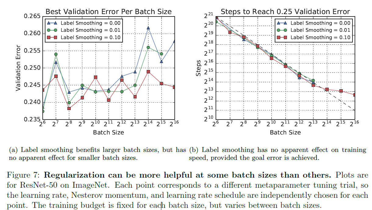
We find no evidence that increasing the batch size necessarily degrades model quality, but additional regularization techniques may become important at larger batch sizes.
-
- Related Work
-
batching cannot hurt the asymptotic guarantees of steps to convergence(上面两篇论文不是说,对收敛有害,容易陷入局部极小值么?), but it could be wasteful of examples. The two extremes imply radically different guidance for practitioners, so the critical task of establishing a relationship between batch size and number of training steps remains one to resolve experimentally.
-
- Experiments and Results
- 实验设置
-
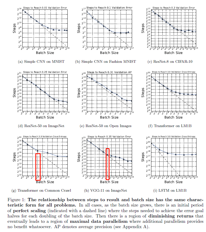
The primary quantity we measure is the number of steps needed to firrst reach a desired out-of-sample error, or steps to result(注意,是提前设置一个损失函数目标,而不是要到收敛).
-
- Steps to Result Depends on Batch Size in a Similar Way Across Problems
![]()
- Some Models Can Exploit Much Larger Batch Sizes Than Others
![]()
-
in Figure 3f, the curves for narrower Transformer models on LM1B atten later than for wider Transformer models, while the depth seems to have less of an effect. Thus, reducing width appears to allow Transformer to make more use of larger batch sizes on LM1B.
-
Momentum Extends Perfect Scaling to Larger Batch Sizes, but Matches Plain SGD at Small Batch Sizes
![]()
- Regularization Can Be More Helpful at Some Batch Sizes Than Others
![]()
![]()
- Regularization Can Be More Helpful at Some Batch Sizes Than Others
![]()
- The Best Learning Rate and Momentum Vary with Batch Size
![]()
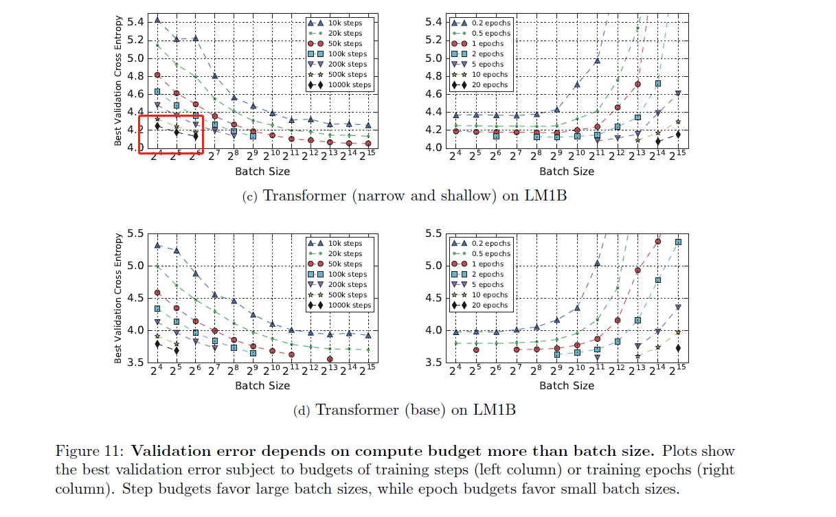
- Solution Quality Depends on Compute Budget More Than Batch Size
![]()
- Discussion
- Our results indicate that, for idealized data parallel hardware, there is a universal relationship between training time and batch size, but there is dramatic variation in how well different workloads can make use of larger batch sizes.
- On the one hand, the possibility that perfect scaling can extend to batch sizes beyond 2^13 for some workloads is good news for practitioners because it suggests that effcient data-parallel systems can provide extremely large speedups for neural network training. On the other hand, the wide variation in scaling behavior across workloads is bad newsbecause any given workload might have a maximum useful batch size well below the limits of our hardware.
- We were unable to find reliable support for any of the previously proposed heuristics for adjusting the learning rate as a function of batch size. Thus we are forced to recommend that practitioners tune all optimization parametersanew when they change the batch size or they risk masking the true behavior of the training procedure.
- 实验设置
4. Scaling Laws for Neural Language Models(Require, 2020, Johns Hopkins University, OpenAI)
- 动机
- One might expect language modeling performance to depend on model architecture, the size of neural models, the computing power used to train them, and the data available for this training process. In this work we will empirically investigate the dependence of language modeling loss on all of these factors, focusing on the Transformer architecture
- Introduction
- Summary
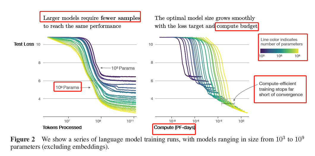
- Performance depends strongly on scale, weakly on model shape: Model performance depends most strongly on scale, which consists of three factors: the number of model parameters N (excluding embeddings), the size of the dataset D, and the amount of compute C used for training
- Performance has a power-law relationship with each of the three scale factors N;D;C when not bottlenecked by the other two, with trends spanning more than six orders of magnitude
- Universality of overfitting: Performance improves predictably as long as we scale up N and D in tandem(协同地), but enters a regime of diminishing returns if either N or D is held fixed while the other increases. The performance penalty depends predictably on the ratio N^0.74/D, meaning that every time we increase the model size 8x, we only need to increase the data by roughly 5x to avoid a penalty
-
Universality of training: Training curves follow predictable power-laws whose parameters are roughly independent of the model size. By extrapolating the early part of a training curve, we can roughly predict the loss that would be achieved if we trained for much longer.
-
Transfer improves with test performance: When we evaluate models on text with a different distribution than they were trained on, the results are strongly correlated to those on the training validation set with a roughly constant offset in the loss – in other words, transfer to a different distribution incurs a constant penalty but otherwise improves roughly in line with performance on the training set
-
Sample efficiency: Large models are more sample-efficient than small models, reaching the same level of performance with fewer optimization steps and using fewer data points
![]()
-
Convergence is inefficient: When working within a fixed compute budget C but without any other restrictions on the model size N or available data D, we attain optimal performance by training very large modelsand stopping significantly short of convergence(远未收敛)
-
Optimal batch size: The ideal batch size for training these models is roughly a power of the loss only, and continues to be determinable by measuring the gradient noise scale ; it is roughly 1-2 million tokens at convergence for the largest models we can train.
- Summary
- Background and Methods
- Empirical Results and Basic Power Laws
5. Scaling Vision Transformers(Optional 2022, Google)
- 动机
-
While the laws for scaling Transformer language models have been studied(上篇), it is unknown how Vision Transformers scale.
-
- 工作:
-
we experiment with models ranging from five million to two billion parameters, datasets ranging from one million to three billion training images and compute budgets ranging from below one TPUv3 core-day to beyond 10 000 core-days.
-
We investigate training hyper-parameters and discover subtle choices that make drastic improvements in few-shot transfer performance
-
we discover that very strong L2 regularization, applied to the final linear prediction layer only, results in a learned visual representation that has very strong few-shot transfer capabilities. For example, with just a single example per class on the ImageNet dataset (which has 1 000 classes), our best model achieves 69.52% accuracy; and with 10 examples per class it attains 84.86%
-
we substantially reduce the memory footprint of the original ViT model proposed in [16]. We achieve this by hardware-specific architecture changes and a different optimizer
-
-
- Core Results
- Scaling up compute, model and data together
![]()
-
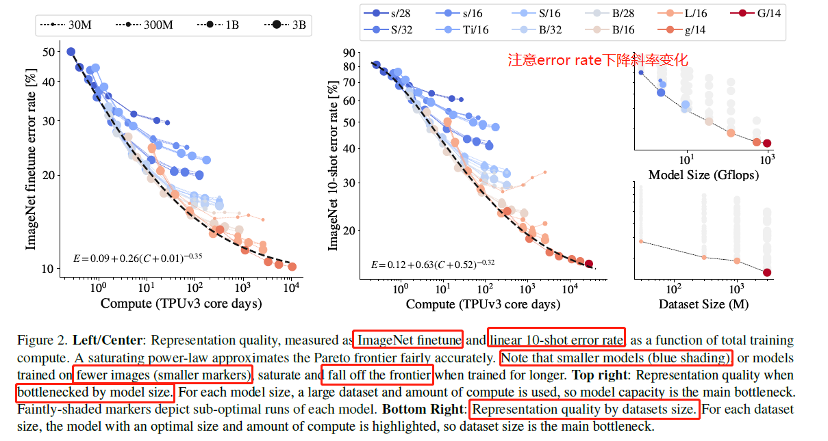
scaling up compute, model and data together improves representation quality
-
representation quality can be bottlenecked by model size
-
large models benefit from additional data, even beyond 1B images
-
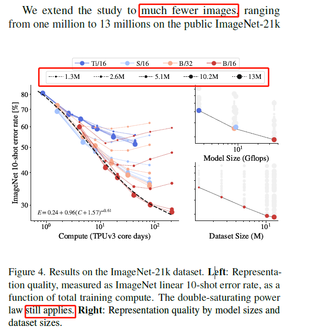
Doublesaturating power law
- E = a(C + d)^b + c
- For over two orders of magnitude of compute, the relationship between compute and performance follows a power-law(E = aC^b)
-
At the higher end of compute, the largest models do not tend towards zero error-rate. In terms of the law, this saturation corresponds to an additive constant to the error rate: c in E = aC^b + c
-
At the lower end of the compute spectrum, we see a saturation for smaller models; the performance of the smallest model is better than that would be predicted by a power-law. This saturation corresponds to a shift in the x axis: d in E = a(C + d)^b + c
- E = a(C + d)^b + c
- Big models are more sample efficient
-
We observe that bigger models are more sample efficient, reaching the same level of error rate with fewer seen images. Our results suggest that with sufficient data, training a larger model for fewer steps is preferable
-
- Do scaling laws still apply on fewer images
![]()
-
2.5. ViTG/14 results
-
We trained a large Vision Transformer, ViT-G/14, which contains nearly two billion parameters
-
-
Method details(train ViT-G/14 using data-parallelism alone, with the entire model fitting on a single TPUv3 core.)
-
Decoupled weight decay for the “head”
-
we observe that high weight decay in the head decreases performance on the pre-training (upstream) task (not shown), despite improving transfer performance
-
we hypothesize that a stronger weight decay in the head results in representations with larger margin between classes, and thus better few-shot adaptation
-
-
Saving memory by removing [class] token
-
The largest VIT model from [16] uses 14 * 14 patches with 224 * 224 images. This results in 256 visual “tokens”, where each one corresponds to an image patch. On top of this, ViT models have an extra [class] token, which is used to produce the final representation, bringing the total number of tokens to 257. For ViT models, current TPU hardware pads the token dimension to a multiple of 128, which may result in up to a 50% memory overhead
-
multihead attention pooling (MAP) [25] to aggregate representation from all patch tokens
-
-
Scaling up data
-
Memoryefficient optimizers
-
the Adam optimizer that is commonly used for training Transformers, stores two additional floating point scalars per each parameter, which results in an additional two-fold overhead
-
We empirically observe that storing momentum in half-precision (bfloat16 type) does not affect training dynamics and has no effect on the outcome. This allows to reduce optimizer overhead from 2-fold to 1.5-fold
-
-
Adafactor optimizer [35], which stores second momentum using rank 1 factorization. From practical point of view, this results in the negligible memory overhead. However, the Adafactor optimizer did not work out of the box, so we make the following modifications
-
-
Learningrate schedule
-
we want to train each of the models for several different durations in order to measure the tradeoff between model size and training duration. When using linear decay, as in [16], each training duration requires its own training run starting from scratch, which would be an inefficient protocol.(如果每个模型,每个duration都从头训练,极大浪费)
-
we address this issue by exploring learning-rate schedules that, similar to the warmup phase in the beginning, include a cooldown phase at the end of training, where the learning-rate is linearly annealed toward zero. Between the warmup and the cooldown phases, the
learning-rate should not decay too quickly to zero
-
-
- Scaling up compute, model and data together
6. Train Large, Then Compress: Rethinking Model Size for Efficient Training and Inference of Transformers(Optional2020)
- 动机
-
This constraint causes the (often implicit) goal of model training to be maximizing compute efficiency: how to achieve the highest model accuracy given a fixed amount of hardware and training time
-
analyze when and why large models train fast and compress well
-
- Experimental Setup
- Tasks, Models, and Datasets
- Self-supervised Pretraining (MLM), We closely follow the pretraining setup and model from ROBERTA (Liu et al.,2019b) with a few minor exceptions.
-
Machine Translation For machine translation (MT) we train the standard Transformer architecture and hyperparameterson the WMT14 English!French dataset
- Evaluation Metrics: FLOPs and Wall-Clock Time
-
We instead directly report wall-clock time as our main evaluation metric. Since the runtime varies across machines (the hardware setups are different, the jobs are not isolated, etc.), we use a single machine to benchmark the timeper-gradient step for each model size. In particular, we train models and wait for the time per gradient step to stabilize, and then we use the average time over 100 steps to calculate the training duration.
-
- Tasks, Models, and Datasets
- Larger Models Train Faster
- Increase Model Width and Sometimes Depth
-
increasing either the width or the depth is effective at accelerating model training. On the other hand, the preferred way to scale models for MT is to increase their width as wider models usually outperform deep models in final performance
-
- Larger Models Are Not Harder to Finetune
-
All models reach comparable accuracies (in fact, the larger models typically outperform the smaller ones), which shows that larger models are not more difficult to finetune.
-
- Increase Model Width and Sometimes Depth
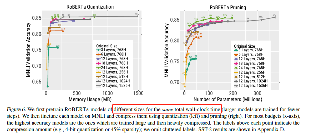
- Larger Models Compress Better
- Larger Models Are More Robust to Quantization
![]()
-
The larger models are more robust to quantization than the smaller models (the accuracy drop is smaller when the precision is reduced). Hence, the models which are trained using large parameter counts and then heavily quantized achieve the highest accuracy for almost all memory budgets.
- Larger Models Are More Robust to Pruning
-
-
Concretely, we consider models with sparsity levels of 15%, 30%, 45%, 60%, 75%, and 90%. We first find the 15% of weights with the smallest magnitude and set them to zero.6 We then finetune the model on the downstream task until it reaches within 99.5% of its original validation accuracy or until we reach one training epoch. We then repeat this process—we prune another 15% of the smallest magnitude weights and finetune—stopping when we reach the desired sparsity level. The additional training overhead from this iterative
process is small because the model typically recovers its accuracy in significantly less than one epoch (sometimes it does not require any retraining to maintain 99.5%).
-
-
- Combining Quantization and Pruning Results
-
-
A particularly strong compression method is to prune 30-40% of the weights and then quantize the model to 6-8 bits.
-
-
- Larger Models Are More Robust to Quantization
- When and Why Are Larger Models Better
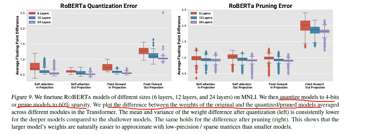
- Smaller Compression Error for Larger Models
-
We first measure the quantization error—the difference between the full-precision and low-precision weights—for the 4-bit ROBERTA models. The mean and variance of the quantization error are smaller for deeper models.
![]()
-
- Smaller Compression Error for Larger Models
7. Deep Learning Training in Facebook Data Centers:Design of Scale-up and Scale-out(超出范围之外) Systems
- 动机
-
Across a period of 18 months, there has been over 4 times increase in the amount of computer resources utilized by training workloads
-
Prior training platform from Facebook, e.g. Big Basin [31], consisted of NVidia GPUs. However, it did not leverage other accelerators and only had support for a limited number of CPUs.
-
- 工作
- On the other hand, the Zion next-generation training platform incorporates 8 CPU sockets, with a modular design having separate sub-components for CPUs (Angels Landing 8- socket system) and accelerators (Emeralds Pools 8-accelerator system). This provides for sufficient general purpose compute and more importantly, additional memory capacity
-
Zion also introduced the common form factor OCP Accelerator Module (OAM) [49]1, which has been adopted by leading GPU vendors such as NVidia。 This is important for enabling consumers such Facebook to build vendor agnostic(无关) accelerator based systems.
- BACKGROUND
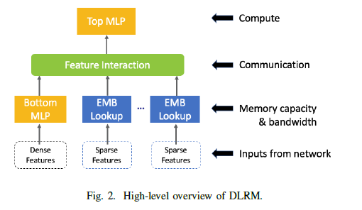
- Recommendation Model
-
The inputs to the recommendation model include both dense and sparse features. The dense or the continuous features are processed with a bottom multilayer perceptron (MLP) while the sparse or the categorical features are processed using embeddings. The second-order interactions of different features are computed explicitly. Finally, the results are processed with a top MLP and fed into a sigmoid function in order to provide a probability of a click.
![]()
![]()
-
- Distributed Training
- Recommendation Model
- TRAINING AT FACEBOOK
- Overview of Training at Facebook
- Synchronous training
-
The compute intensive MLPs are replicated across devices and work on parts of the mini-batch data samples(数据并行). Notice that training of MLPs requires an allreduce communication primitive to synchronize their weights during backward propagation
-
Further, a model may contain tens of embedding tables, which can not be replicated due to memory capacity constraints. These tables are often distributed across devices and each of them processes an entire mini-batch of lookups. Then, an embedding lookup produces several vectors corresponding to the elements in the mini-batch. Let us use the same color to denote vectors resulting from a single embedding table. The need to exchange these vectors in the forward pass and their gradients in the backward pass gives rise to the alltoallcommunication primitive
-
In this setting, embedding lookups take advantage of the aggregate memory bandwidth across devices
-
-
Asynchronous training is well suited for a disaggregated(分解) design with use of dedicated parameter servers and trainers, that are relying on point-to-point send/recv communication or Remote Procedure Calls (RPC)
-
The compute intensive MLPs are replicated on different training processes and perform local weights updates based on the data samples they receive individually, only occasionally synchronizing with a master copy of the weights stored on the parameter server.
-
- Synchronous training
- Scalability & Challenges
-
we use asynchronous training to avoid being bottlenecked by slow machines and/or interconnects. Also, we make sure the synchronization of the dense parameters is frequent enough, so that models will not diverge on different machines
-
asynchronous training works well when a limited number of trainers is used, but with increasing number of trainers, we must incorporate synchronous training as an option into our system and hardware platforms
-
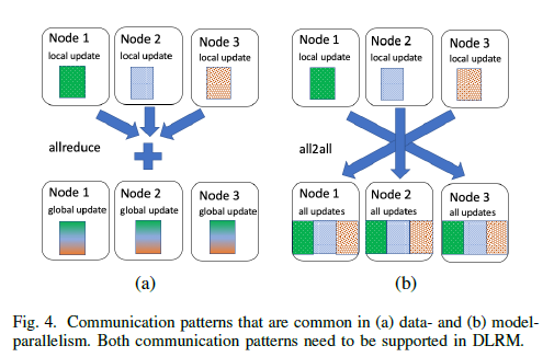
- Interconnection Networks
-
Aside from the standard send/recv communication primitives, the data- and model-parallelism used in distributed training give rise to two types of communication patterns: (i) allreduce operation that is often used to aggregate local parameter updates in the backward pass and (ii) alltoall operation that can be used to exchange the activations and error gradients across multiple nodes with different model weights.
-
- Overview of Training at Facebook

 浙公网安备 33010602011771号