Deep SORT多目标跟踪算法代码解析

Deep SORT是多目标跟踪(Multi-Object Tracking)中常用到的一种算法，是一个Detection Based Tracking的方法。这个算法工业界关注度非常高，在知乎上有很多文章都是使用了Deep SORT进行工程部署。笔者将参考前辈的博客，结合自己的实践(理论&代码)对Deep SORT算法进行代码层面的解析。

在之前笔者写的一篇Deep SORT论文阅读总结中，总结了DeepSORT论文中提到的核心观点，如果对Deep SORT不是很熟悉，可以先理解一下，然后再来看解读代码的部分。

1. MOT主要步骤

在《DEEP LEARNING IN VIDEO MULTI-OBJECT TRACKING: A SURVEY》这篇基于深度学习的多目标跟踪的综述中，描述了MOT问题中四个主要步骤：

• 给定视频原始帧。
• 运行目标检测器如Faster R-CNN、YOLOv3、SSD等进行检测，获取目标检测框。
• 将所有目标框中对应的目标抠出来，进行特征提取（包括表观特征或者运动特征）。
• 进行相似度计算，计算前后两帧目标之间的匹配程度（前后属于同一个目标的之间的距离比较小，不同目标的距离比较大）
• 数据关联，为每个对象分配目标的ID。

以上就是四个核心步骤，其中核心是检测，SORT论文的摘要中提到，仅仅换一个更好的检测器，就可以将目标跟踪表现提升18.9%。

2. SORT

Deep SORT算法的前身是SORT, 全称是Simple Online and Realtime Tracking。简单介绍一下，SORT最大特点是基于Faster R-CNN的目标检测方法，并利用卡尔曼滤波算法+匈牙利算法，极大提高了多目标跟踪的速度，同时达到了SOTA的准确率。

这个算法确实是在实际应用中使用较为广泛的一个算法，核心就是两个算法：卡尔曼滤波和匈牙利算法。

卡尔曼滤波算法分为两个过程，预测和更新。该算法将目标的运动状态定义为8个正态分布的向量。

预测：当目标经过移动，通过上一帧的目标框和速度等参数，预测出当前帧的目标框位置和速度等参数。

更新：预测值和观测值，两个正态分布的状态进行线性加权，得到目前系统预测的状态。

匈牙利算法：解决的是一个分配问题，在MOT主要步骤中的计算相似度的，得到了前后两帧的相似度矩阵。匈牙利算法就是通过求解这个相似度矩阵，从而解决前后两帧真正匹配的目标。这部分sklearn库有对应的函数linear_assignment来进行求解。

SORT算法中是通过前后两帧IOU来构建相似度矩阵，所以SORT计算速度非常快。

下图是一张SORT核心算法流程图：

Detections是通过目标检测器得到的目标框，Tracks是一段轨迹。核心是匹配的过程与卡尔曼滤波的预测和更新过程。

流程如下：目标检测器得到目标框Detections，同时卡尔曼滤波器预测当前的帧的Tracks, 然后将Detections和Tracks进行IOU匹配，最终得到的结果分为：

• Unmatched Tracks，这部分被认为是失配，Detection和Track无法匹配，如果失配持续了\(T_{lost}\)次，该目标ID将从图片中删除。
• Unmatched Detections, 这部分说明没有任意一个Track能匹配Detection, 所以要为这个detection分配一个新的track。
• Matched Track，这部分说明得到了匹配。

卡尔曼滤波可以根据Tracks状态预测下一帧的目标框状态。

卡尔曼滤波更新是对观测值(匹配上的Track)和估计值更新所有track的状态。

3. Deep SORT

DeepSort中最大的特点是加入外观信息，借用了ReID领域模型来提取特征，减少了ID switch的次数。整体流程图如下：

可以看出，Deep SORT算法在SORT算法的基础上增加了级联匹配(Matching Cascade)+新轨迹的确认(confirmed)。总体流程就是：

• 卡尔曼滤波器预测轨迹Tracks
• 使用匈牙利算法将预测得到的轨迹Tracks和当前帧中的detections进行匹配(级联匹配和IOU匹配)
• 卡尔曼滤波更新。

其中上图中的级联匹配展开如下：

上图非常清晰地解释了如何进行级联匹配，上图由虚线划分为两部分：

上半部分中计算相似度矩阵的方法使用到了外观模型(ReID)和运动模型(马氏距离)来计算相似度，得到代价矩阵，另外一个则是门控矩阵，用于限制代价矩阵中过大的值。

下半部分中是是级联匹配的数据关联步骤，匹配过程是一个循环(max age个迭代，默认为70)，也就是从missing age=0到missing age=70的轨迹和Detections进行匹配，没有丢失过的轨迹优先匹配，丢失较为久远的就靠后匹配。通过这部分处理，可以重新将被遮挡目标找回，降低被遮挡然后再出现的目标发生的ID Switch次数。

将Detection和Track进行匹配，所以出现几种情况

1. Detection和Track匹配，也就是Matched Tracks。普通连续跟踪的目标都属于这种情况，前后两帧都有目标，能够匹配上。
2. Detection没有找到匹配的Track，也就是Unmatched Detections。图像中突然出现新的目标的时候，Detection无法在之前的Track找到匹配的目标。
3. Track没有找到匹配的Detection，也就是Unmatched Tracks。连续追踪的目标超出图像区域，Track无法与当前任意一个Detection匹配。
4. 以上没有涉及一种特殊的情况，就是两个目标遮挡的情况。刚刚被遮挡的目标的Track也无法匹配Detection，目标暂时从图像中消失。之后被遮挡目标再次出现的时候，应该尽量让被遮挡目标分配的ID不发生变动，减少ID Switch出现的次数，这就需要用到级联匹配了。

4. Deep SORT代码解析

论文中提供的代码是如下地址: https://github.com/nwojke/deep_sort

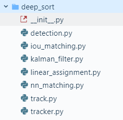
上图是Github库中有关Deep SORT的核心代码，不包括Faster R-CNN检测部分，所以主要将讲解这部分的几个文件，笔者也对其中核心代码进行了部分注释，地址在: https://github.com/pprp/deep_sort_yolov3_pytorch , 将其中的目标检测器换成了U版的yolov3, 将deep_sort文件中的核心进行了调用。

4.1 类图

下图是笔者总结的这几个类调用的类图(不是特别严谨，但是能大概展示各个模块的关系)：

DeepSort是核心类，调用其他模块，大体上可以分为三个模块：

• ReID模块，用于提取表观特征，原论文中是生成了128维的embedding。
• Track模块，轨迹类，用于保存一个Track的状态信息，是一个基本单位。
• Tracker模块，Tracker模块掌握最核心的算法，卡尔曼滤波和匈牙利算法都是通过调用这个模块来完成的。

DeepSort类对外接口非常简单：

self.deepsort = DeepSort(args.deepsort_checkpoint)#实例化
outputs = self.deepsort.update(bbox_xcycwh, cls_conf, im)#通过接收目标检测结果进行更新

在外部调用的时候只需要以上两步即可，非常简单。

通过类图，对整体模块有了框架上理解，下面深入理解一下这些模块。

4.2 核心模块

Detection类

class Detection(object):
    """
    This class represents a bounding box detection in a single image.
	"""
    def __init__(self, tlwh, confidence, feature):
        self.tlwh = np.asarray(tlwh, dtype=np.float)
        self.confidence = float(confidence)
        self.feature = np.asarray(feature, dtype=np.float32)
    def to_tlbr(self):
        """Convert bounding box to format `(min x, min y, max x, max y)`, i.e.,
        `(top left, bottom right)`.
        """
        ret = self.tlwh.copy()
        ret[2:] += ret[:2]
        return ret
    def to_xyah(self):
        """Convert bounding box to format `(center x, center y, aspect ratio,
        height)`, where the aspect ratio is `width / height`.
        """
        ret = self.tlwh.copy()
        ret[:2] += ret[2:] / 2
        ret[2] /= ret[3]
        return ret

Detection类用于保存通过目标检测器得到的一个检测框，包含top left坐标+框的宽和高，以及该bbox的置信度还有通过reid获取得到的对应的embedding。除此以外提供了不同bbox位置格式的转换方法：

• tlwh: 代表左上角坐标+宽高
• tlbr: 代表左上角坐标+右下角坐标
• xyah: 代表中心坐标+宽高比+高

Track类

class Track:
    # 一个轨迹的信息，包含(x,y,a,h) & v
    """
    A single target track with state space `(x, y, a, h)` and associated
    velocities, where `(x, y)` is the center of the bounding box, `a` is the
    aspect ratio and `h` is the height.
    """

    def __init__(self, mean, covariance, track_id, n_init, max_age,
                 feature=None):
        # max age是一个存活期限，默认为70帧,在
        self.mean = mean
        self.covariance = covariance
        self.track_id = track_id
        self.hits = 1 
        # hits和n_init进行比较
        # hits每次update的时候进行一次更新（只有match的时候才进行update）
        # hits代表匹配上了多少次，匹配次数超过n_init就会设置为confirmed状态
        self.age = 1 # 没有用到，和time_since_update功能重复
        self.time_since_update = 0
        # 每次调用predict函数的时候就会+1
        # 每次调用update函数的时候就会设置为0

        self.state = TrackState.Tentative
        self.features = []
        # 每个track对应多个features, 每次更新都将最新的feature添加到列表中
        if feature is not None:
            self.features.append(feature)

        self._n_init = n_init  # 如果连续n_init帧都没有出现失配，设置为deleted状态
        self._max_age = max_age  # 上限

Track类主要存储的是轨迹信息，mean和covariance是保存的框的位置和速度信息，track_id代表分配给这个轨迹的ID。state代表框的状态，有三种：

• Tentative: 不确定态，这种状态会在初始化一个Track的时候分配，并且只有在连续匹配上n_init帧才会转变为确定态。如果在处于不确定态的情况下没有匹配上任何detection，那将转变为删除态。
• Confirmed: 确定态，代表该Track确实处于匹配状态。如果当前Track属于确定态，但是失配连续达到max age次数的时候，就会被转变为删除态。
• Deleted: 删除态，说明该Track已经失效。

max_age代表一个Track存活期限，他需要和time_since_update变量进行比对。time_since_update是每次轨迹调用predict函数的时候就会+1，每次调用predict的时候就会重置为0，也就是说如果一个轨迹长时间没有update(没有匹配上)的时候，就会不断增加，直到time_since_update超过max age(默认70)，将这个Track从Tracker中的列表删除。

hits代表连续确认多少次，用在从不确定态转为确定态的时候。每次Track进行update的时候，hits就会+1, 如果hits>n_init(默认为3)，也就是连续三帧的该轨迹都得到了匹配，这时候才将不确定态转为确定态。

需要说明的是每个轨迹还有一个重要的变量，features列表，存储该轨迹在不同帧对应位置通过ReID提取到的特征。为何要保存这个列表，而不是将其更新为当前最新的特征呢？这是为了解决目标被遮挡后再次出现的问题，需要从以往帧对应的特征进行匹配。另外，如果特征过多会严重拖慢计算速度，所以有一个参数budget用来控制特征列表的长度，取最新的budget个features,将旧的删除掉。

ReID特征提取部分

ReID网络是独立于目标检测和跟踪器的模块，功能是提取对应bounding box中的feature,得到一个固定维度的embedding作为该bbox的代表，供计算相似度时使用。

class Extractor(object):
    def __init__(self, model_name, model_path, use_cuda=True):
        self.net = build_model(name=model_name,
                               num_classes=96)
        self.device = "cuda" if torch.cuda.is_available(
        ) and use_cuda else "cpu"
        state_dict = torch.load(model_path)['net_dict']
        self.net.load_state_dict(state_dict)
        print("Loading weights from {}... Done!".format(model_path))
        self.net.to(self.device)
        self.size = (128,128)
        self.norm = transforms.Compose([
            transforms.ToTensor(),
            transforms.Normalize([0.3568, 0.3141, 0.2781],
                                 [0.1752, 0.1857, 0.1879])
        ])

    def _preprocess(self, im_crops):
        """
        TODO:
            1. to float with scale from 0 to 1
            2. resize to (64, 128) as Market1501 dataset did
            3. concatenate to a numpy array
            3. to torch Tensor
            4. normalize
        """
        def _resize(im, size):
            return cv2.resize(im.astype(np.float32) / 255., size)

        im_batch = torch.cat([
            self.norm(_resize(im, self.size)).unsqueeze(0) for im in im_crops
        ],dim=0).float()
        return im_batch

    def __call__(self, im_crops):
        im_batch = self._preprocess(im_crops)
        with torch.no_grad():
            im_batch = im_batch.to(self.device)
            features = self.net(im_batch)
        return features.cpu().numpy()

模型训练是按照传统ReID的方法进行，使用Extractor类的时候输入为一个list的图片，得到图片对应的特征。

NearestNeighborDistanceMetric类

这个类中用到了两个计算距离的函数：

1. 计算欧氏距离

def _pdist(a, b):
    # 用于计算成对的平方距离
    # a NxM 代表N个对象，每个对象有M个数值作为embedding进行比较
    # b LxM 代表L个对象，每个对象有M个数值作为embedding进行比较
    # 返回的是NxL的矩阵，比如dist[i][j]代表a[i]和b[j]之间的平方和距离
    # 实现见：https://blog.csdn.net/frankzd/article/details/80251042
    a, b = np.asarray(a), np.asarray(b)  # 拷贝一份数据
    if len(a) == 0 or len(b) == 0:
        return np.zeros((len(a), len(b)))
    a2, b2 = np.square(a).sum(axis=1), np.square(
        b).sum(axis=1)  # 求每个embedding的平方和
    # sum(N) + sum(L) -2 x [NxM]x[MxL] = [NxL]
    r2 = -2. * np.dot(a, b.T) + a2[:, None] + b2[None, :]
    r2 = np.clip(r2, 0., float(np.inf))
    return r2

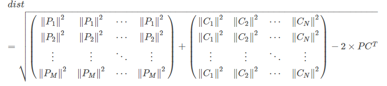
2. 计算余弦距离

def _cosine_distance(a, b, data_is_normalized=False):
    # a和b之间的余弦距离
    # a : [NxM] b : [LxM]
    # 余弦距离 = 1 - 余弦相似度
    # https://blog.csdn.net/u013749540/article/details/51813922
    if not data_is_normalized:
        # 需要将余弦相似度转化成类似欧氏距离的余弦距离。
        a = np.asarray(a) / np.linalg.norm(a, axis=1, keepdims=True)
        #  np.linalg.norm 操作是求向量的范式，默认是L2范式，等同于求向量的欧式距离。
        b = np.asarray(b) / np.linalg.norm(b, axis=1, keepdims=True)
    return 1. - np.dot(a, b.T)

以上代码对应公式，注意余弦距离=1-余弦相似度。

最近邻距离度量类

class NearestNeighborDistanceMetric(object):
    # 对于每个目标，返回一个最近的距离
    def __init__(self, metric, matching_threshold, budget=None):
        # 默认matching_threshold = 0.2 budge = 100
        if metric == "euclidean":
            # 使用最近邻欧氏距离
            self._metric = _nn_euclidean_distance
        elif metric == "cosine":
            # 使用最近邻余弦距离
            self._metric = _nn_cosine_distance
        else:
            raise ValueError("Invalid metric; must be either 'euclidean' or 'cosine'")

        self.matching_threshold = matching_threshold
        # 在级联匹配的函数中调用
        self.budget = budget
        # budge 预算，控制feature的多少
        self.samples = {}
        # samples是一个字典{id->feature list}

    def partial_fit(self, features, targets, active_targets):
        # 作用：部分拟合，用新的数据更新测量距离
        # 调用：在特征集更新模块部分调用，tracker.update()中
        for feature, target in zip(features, targets):
            self.samples.setdefault(target, []).append(feature)
            # 对应目标下添加新的feature，更新feature集合
            # 目标id  :  feature list
            if self.budget is not None:
                self.samples[target] = self.samples[target][-self.budget:]
            # 设置预算，每个类最多多少个目标，超过直接忽略

        # 筛选激活的目标
        self.samples = {k: self.samples[k] for k in active_targets}

    def distance(self, features, targets):
        # 作用：比较feature和targets之间的距离，返回一个代价矩阵
        # 调用：在匹配阶段，将distance封装为gated_metric,
        #       进行外观信息(reid得到的深度特征)+
        #       运动信息(马氏距离用于度量两个分布相似程度)
        cost_matrix = np.zeros((len(targets), len(features)))
        for i, target in enumerate(targets):
            cost_matrix[i, :] = self._metric(self.samples[target], features)
        return cost_matrix

Tracker类

Tracker类是最核心的类，Tracker中保存了所有的轨迹信息，负责初始化第一帧的轨迹、卡尔曼滤波的预测和更新、负责级联匹配、IOU匹配等等核心工作。

class Tracker:
    # 是一个多目标tracker，保存了很多个track轨迹
    # 负责调用卡尔曼滤波来预测track的新状态+进行匹配工作+初始化第一帧
    # Tracker调用update或predict的时候，其中的每个track也会各自调用自己的update或predict
    """
    This is the multi-target tracker.
    """

    def __init__(self, metric, max_iou_distance=0.7, max_age=70, n_init=3):
        # 调用的时候，后边的参数全部是默认的
        self.metric = metric 
        # metric是一个类，用于计算距离(余弦距离或马氏距离)
        self.max_iou_distance = max_iou_distance
        # 最大iou，iou匹配的时候使用
        self.max_age = max_age
        # 直接指定级联匹配的cascade_depth参数
        self.n_init = n_init
        # n_init代表需要n_init次数的update才会将track状态设置为confirmed

        self.kf = kalman_filter.KalmanFilter()# 卡尔曼滤波器
        self.tracks = [] # 保存一系列轨迹
        self._next_id = 1 # 下一个分配的轨迹id
	def predict(self):
        # 遍历每个track都进行一次预测
        """Propagate track state distributions one time step forward.

        This function should be called once every time step, before `update`.
        """
        for track in self.tracks:
            track.predict(self.kf)

然后来看最核心的update函数和match函数，可以对照下面的流程图一起看：

update函数

def update(self, detections):
    # 进行测量的更新和轨迹管理
    """Perform measurement update and track management.

    Parameters
    ----------
    detections : List[deep_sort.detection.Detection]
        A list of detections at the current time step.

    """
    # Run matching cascade.
    matches, unmatched_tracks, unmatched_detections = \
        self._match(detections)

    # Update track set.
    # 1. 针对匹配上的结果
    for track_idx, detection_idx in matches:
        # track更新对应的detection
        self.tracks[track_idx].update(self.kf, detections[detection_idx])

    # 2. 针对未匹配的tracker,调用mark_missed标记
    # track失配，若待定则删除，若update时间很久也删除
    # max age是一个存活期限，默认为70帧
    for track_idx in unmatched_tracks:
        self.tracks[track_idx].mark_missed()

    # 3. 针对未匹配的detection， detection失配，进行初始化
    for detection_idx in unmatched_detections:
        self._initiate_track(detections[detection_idx])

    # 得到最新的tracks列表，保存的是标记为confirmed和Tentative的track
    self.tracks = [t for t in self.tracks if not t.is_deleted()]

    # Update distance metric.
    active_targets = [t.track_id for t in self.tracks if t.is_confirmed()]
    # 获取所有confirmed状态的track id
    features, targets = [], []
    for track in self.tracks:
        if not track.is_confirmed():
            continue
        features += track.features  # 将tracks列表拼接到features列表
        # 获取每个feature对应的track id
        targets += [track.track_id for _ in track.features]
        track.features = []

    # 距离度量中的 特征集更新
    self.metric.partial_fit(np.asarray(features), np.asarray(targets),
                            active_targets)

match函数：

def _match(self, detections):
    # 主要功能是进行匹配，找到匹配的，未匹配的部分
    def gated_metric(tracks, dets, track_indices, detection_indices):
        # 功能： 用于计算track和detection之间的距离，代价函数
        #        需要使用在KM算法之前
        # 调用：
        # cost_matrix = distance_metric(tracks, detections,
        #                  track_indices, detection_indices)
        features = np.array([dets[i].feature for i in detection_indices])
        targets = np.array([tracks[i].track_id for i in track_indices])

        # 1. 通过最近邻计算出代价矩阵 cosine distance
        cost_matrix = self.metric.distance(features, targets)
        # 2. 计算马氏距离,得到新的状态矩阵
        cost_matrix = linear_assignment.gate_cost_matrix(
            self.kf, cost_matrix, tracks, dets, track_indices,
            detection_indices)
        return cost_matrix

    # Split track set into confirmed and unconfirmed tracks.
    # 划分不同轨迹的状态
    confirmed_tracks = [
        i for i, t in enumerate(self.tracks) if t.is_confirmed()
    ]
    unconfirmed_tracks = [
        i for i, t in enumerate(self.tracks) if not t.is_confirmed()
    ]

    # 进行级联匹配，得到匹配的track、不匹配的track、不匹配的detection
    '''
    !!!!!!!!!!!
    级联匹配
    !!!!!!!!!!!
    '''
    # gated_metric->cosine distance
    # 仅仅对确定态的轨迹进行级联匹配
    matches_a, unmatched_tracks_a, unmatched_detections = \
        linear_assignment.matching_cascade(
            gated_metric,
            self.metric.matching_threshold,
            self.max_age,
            self.tracks,
            detections,
            confirmed_tracks)

    # 将所有状态为未确定态的轨迹和刚刚没有匹配上的轨迹组合为iou_track_candidates，
    # 进行IoU的匹配
    iou_track_candidates = unconfirmed_tracks + [
        k for k in unmatched_tracks_a
        if self.tracks[k].time_since_update == 1  # 刚刚没有匹配上
    ]
    # 未匹配
    unmatched_tracks_a = [
        k for k in unmatched_tracks_a
        if self.tracks[k].time_since_update != 1  # 已经很久没有匹配上
    ]

    '''
    !!!!!!!!!!!
    IOU 匹配
    对级联匹配中还没有匹配成功的目标再进行IoU匹配
    !!!!!!!!!!!
    '''
    # 虽然和级联匹配中使用的都是min_cost_matching作为核心，
    # 这里使用的metric是iou cost和以上不同
    matches_b, unmatched_tracks_b, unmatched_detections = \
        linear_assignment.min_cost_matching(
            iou_matching.iou_cost,
            self.max_iou_distance,
            self.tracks,
            detections,
            iou_track_candidates,
            unmatched_detections)

    matches = matches_a + matches_b  # 组合两部分match得到的结果

    unmatched_tracks = list(set(unmatched_tracks_a + unmatched_tracks_b))
    return matches, unmatched_tracks, unmatched_detections

以上两部分结合注释和以下流程图可以更容易理解。

级联匹配

下边是论文中给出的级联匹配的伪代码：

以下代码是伪代码对应的实现

# 1. 分配track_indices和detection_indices
if track_indices is None:
    track_indices = list(range(len(tracks)))

if detection_indices is None:
    detection_indices = list(range(len(detections)))

unmatched_detections = detection_indices

matches = []
# cascade depth = max age 默认为70
for level in range(cascade_depth):
    if len(unmatched_detections) == 0:  # No detections left
        break

    track_indices_l = [
        k for k in track_indices
        if tracks[k].time_since_update == 1 + level
    ]
    if len(track_indices_l) == 0:  # Nothing to match at this level
        continue

    # 2. 级联匹配核心内容就是这个函数
    matches_l, _, unmatched_detections = \
        min_cost_matching(  # max_distance=0.2
            distance_metric, max_distance, tracks, detections,
            track_indices_l, unmatched_detections)
    matches += matches_l
unmatched_tracks = list(set(track_indices) - set(k for k, _ in matches))

门控矩阵

门控矩阵的作用就是通过计算卡尔曼滤波的状态分布和测量值之间的距离对代价矩阵进行限制。

代价矩阵中的距离是Track和Detection之间的表观相似度，假如一个轨迹要去匹配两个表观特征非常相似的Detection，这样就很容易出错，但是这个时候分别让两个Detection计算与这个轨迹的马氏距离，并使用一个阈值gating_threshold进行限制，所以就可以将马氏距离较远的那个Detection区分开，可以降低错误的匹配。

def gate_cost_matrix(
        kf, cost_matrix, tracks, detections, track_indices, detection_indices,
        gated_cost=INFTY_COST, only_position=False):
    # 根据通过卡尔曼滤波获得的状态分布，使成本矩阵中的不可行条目无效。
    gating_dim = 2 if only_position else 4
    gating_threshold = kalman_filter.chi2inv95[gating_dim]  # 9.4877

    measurements = np.asarray([detections[i].to_xyah()
                               for i in detection_indices])
    for row, track_idx in enumerate(track_indices):
        track = tracks[track_idx]
        gating_distance = kf.gating_distance(
            track.mean, track.covariance, measurements, only_position)
        cost_matrix[row, gating_distance >
                    gating_threshold] = gated_cost  # 设置为inf
    return cost_matrix

卡尔曼滤波器

在Deep SORT中，需要估计Track的以下状态：

• 均值：用8维向量（x, y, a, h, vx, vy, va, vh）表示。(x,y)是框的中心坐标，宽高比是a, 高度h以及对应的速度，所有的速度都将初始化为0。
• 协方差：表示目标位置信息的不确定程度，用8x8的对角矩阵来表示，矩阵对应的值越大，代表不确定程度越高。

下图代表卡尔曼滤波器主要过程：

1. 卡尔曼滤波首先根据当前帧(time=t)的状态进行预测，得到预测下一帧的状态(time=t+1)
2. 得到测量结果，在Deep SORT中对应的测量就是Detection，即目标检测器提供的检测框。
3. 将预测结果和测量结果进行更新。

下面这部分主要参考： https://zhuanlan.zhihu.com/p/90835266

如果对卡尔曼滤波算法有较为深入的了解，可以结合卡尔曼滤波算法和代码进行理解。

预测分两个公式：

第一个公式：

\[x'=Fx \]

其中F是状态转移矩阵，如下图：

第二个公式：

\[P'=FPF^T+Q \]

P是当前帧(time=t)的协方差，Q是卡尔曼滤波器的运动估计误差，代表不确定程度。

def predict(self, mean, covariance):
    # 相当于得到t时刻估计值
    # Q 预测过程中噪声协方差
    std_pos = [
        self._std_weight_position * mean[3],
        self._std_weight_position * mean[3],
        1e-2,
        self._std_weight_position * mean[3]]

    std_vel = [
        self._std_weight_velocity * mean[3],
        self._std_weight_velocity * mean[3],
        1e-5,
        self._std_weight_velocity * mean[3]]

    # np.r_ 按列连接两个矩阵
    # 初始化噪声矩阵Q
    motion_cov = np.diag(np.square(np.r_[std_pos, std_vel]))

    # x' = Fx
    mean = np.dot(self._motion_mat, mean)

    # P' = FPF^T+Q
    covariance = np.linalg.multi_dot((
        self._motion_mat, covariance, self._motion_mat.T)) + motion_cov

    return mean, covariance

更新的公式

\[y=z-Hx' \\ \]

\[S=HP'H^T+R \\ \]

\[K=P'H^TS^{-1} \\ \]

\[x=x'+Ky \\ \]

\[P=(I-KH)P' \]

def project(self, mean, covariance):
    # R 测量过程中噪声的协方差
    std = [
        self._std_weight_position * mean[3],
        self._std_weight_position * mean[3],
        1e-1,
        self._std_weight_position * mean[3]]

    # 初始化噪声矩阵R
    innovation_cov = np.diag(np.square(std))

    # 将均值向量映射到检测空间，即Hx'
    mean = np.dot(self._update_mat, mean)

    # 将协方差矩阵映射到检测空间，即HP'H^T
    covariance = np.linalg.multi_dot((
        self._update_mat, covariance, self._update_mat.T))

    return mean, covariance + innovation_cov

def update(self, mean, covariance, measurement):
    # 通过估计值和观测值估计最新结果

    # 将均值和协方差映射到检测空间，得到 Hx' 和 S
    projected_mean, projected_cov = self.project(mean, covariance)

    # 矩阵分解
    chol_factor, lower = scipy.linalg.cho_factor(
        projected_cov, lower=True, check_finite=False)

    # 计算卡尔曼增益K
    kalman_gain = scipy.linalg.cho_solve(
        (chol_factor, lower), np.dot(covariance, self._update_mat.T).T,
        check_finite=False).T

    # z - Hx'
    innovation = measurement - projected_mean

    # x = x' + Ky
    new_mean = mean + np.dot(innovation, kalman_gain.T)

    # P = (I - KH)P'
    new_covariance = covariance - np.linalg.multi_dot((
        kalman_gain, projected_cov, kalman_gain.T))
    return new_mean, new_covariance

\[y=z-Hx' \]

这个公式中，z是Detection的mean，不包含变化值，状态为[cx,cy,a,h]。H是测量矩阵，将Track的均值向量\(x'\)映射到检测空间。计算的y是Detection和Track的均值误差。

\[S=HP'H^T+R \]

R是目标检测器的噪声矩阵，是一个4x4的对角矩阵。 对角线上的值分别为中心点两个坐标以及宽高的噪声。

\[K=P'H^TS^{-1} \]

计算的是卡尔曼增益，是作用于衡量估计误差的权重。

\[x=x'+Ky \]

更新后的均值向量x。

\[P=(I-KH)P' \]

更新后的协方差矩阵。

卡尔曼滤波笔者理解也不是很深入，没有推导过公式，对这部分感兴趣的推荐几个博客：

1. 卡尔曼滤波+python写的demo: https://zhuanlan.zhihu.com/p/113685503?utm_source=wechat_session&utm_medium=social&utm_oi=801414067897135104
2. 详解+推导： https://blog.csdn.net/honyniu/article/details/88697520

5. 流程解析

流程部分主要按照以下流程图来走一遍：

感谢知乎@猫弟总结的流程图，讲解非常地清晰，如果单纯看代码，非常容易混淆。比如说代价矩阵的计算这部分，连续套了三个函数，才被真正调用。上图将整体流程总结地非常棒。笔者将参考以上流程结合代码进行梳理：

1. 分析detector类中的Deep SORT调用：

class Detector(object):
    def __init__(self, args):
        self.args = args
        if args.display:
            cv2.namedWindow("test", cv2.WINDOW_NORMAL)
            cv2.resizeWindow("test", args.display_width, args.display_height)

        device = torch.device(
            'cuda') if torch.cuda.is_available() else torch.device('cpu')

        self.vdo = cv2.VideoCapture()
        self.yolo3 = InferYOLOv3(args.yolo_cfg,
                                 args.img_size,
                                 args.yolo_weights,
                                 args.data_cfg,
                                 device,
                                 conf_thres=args.conf_thresh,
                                 nms_thres=args.nms_thresh)
        self.deepsort = DeepSort(args.deepsort_checkpoint)

初始化DeepSORT对象，更新部分接收目标检测得到的框的位置，置信度和图片：

outputs = self.deepsort.update(bbox_xcycwh, cls_conf, im)

2. 顺着DeepSORT类的update函数看

class DeepSort(object):
    def __init__(self, model_path, max_dist=0.2):
        self.min_confidence = 0.3
        # yolov3中检测结果置信度阈值，筛选置信度小于0.3的detection。

        self.nms_max_overlap = 1.0
        # 非极大抑制阈值，设置为1代表不进行抑制

        # 用于提取图片的embedding,返回的是一个batch图片对应的特征
        self.extractor = Extractor("resnet18",
                                   model_path,
                                   use_cuda=True)

        max_cosine_distance = max_dist
        # 用在级联匹配的地方，如果大于改阈值，就直接忽略
        nn_budget = 100
        # 预算，每个类别最多的样本个数，如果超过，删除旧的

        # 第一个参数可选'cosine' or 'euclidean'
        metric = NearestNeighborDistanceMetric("cosine",
                                               max_cosine_distance,
                                               nn_budget)
        self.tracker = Tracker(metric)

    def update(self, bbox_xywh, confidences, ori_img):
        self.height, self.width = ori_img.shape[:2]
        # generate detections
        features = self._get_features(bbox_xywh, ori_img)
        # 从原图中crop bbox对应图片并计算得到embedding
        bbox_tlwh = self._xywh_to_tlwh(bbox_xywh)

        detections = [
            Detection(bbox_tlwh[i], conf, features[i])
            for i, conf in enumerate(confidences) if conf > self.min_confidence
        ]  # 筛选小于min_confidence的目标，并构造一个Detection对象构成的列表
        # Detection是一个存储图中一个bbox结果
        # 需要：1. bbox(tlwh形式) 2. 对应置信度 3. 对应embedding

        # run on non-maximum supression
        boxes = np.array([d.tlwh for d in detections])
        scores = np.array([d.confidence for d in detections])

        # 使用非极大抑制
        # 默认nms_thres=1的时候开启也没有用，实际上并没有进行非极大抑制
        indices = non_max_suppression(boxes, self.nms_max_overlap, scores)
        detections = [detections[i] for i in indices]

        # update tracker
        # tracker给出一个预测结果，然后将detection传入，进行卡尔曼滤波操作
        self.tracker.predict()
        self.tracker.update(detections)

        # output bbox identities
        # 存储结果以及可视化
        outputs = []
        for track in self.tracker.tracks:
            if not track.is_confirmed() or track.time_since_update > 1:
                continue
            box = track.to_tlwh()
            x1, y1, x2, y2 = self._tlwh_to_xyxy(box)
            track_id = track.track_id
            outputs.append(np.array([x1, y1, x2, y2, track_id], dtype=np.int))

        if len(outputs) > 0:
            outputs = np.stack(outputs, axis=0)
        return np.array(outputs)

从这里开始对照以上流程图会更加清晰。在Deep SORT初始化的过程中有一个核心metric，NearestNeighborDistanceMetric类会在匹配和特征集更新的时候用到。

梳理DeepSORT的update流程：

• 根据传入的参数（bbox_xywh, conf, img）使用ReID模型提取对应bbox的表观特征。

• 构建detections的列表，列表中的内容就是Detection类,在此处限制了bbox的最小置信度。

• 使用非极大抑制算法，由于默认nms_thres=1，实际上并没有用。

• Tracker类进行一次预测，然后将detections传入，进行更新。

• 最后将Tracker中保存的轨迹中状态属于确认态的轨迹返回。

以上核心在Tracker的predict和update函数，接着梳理。

3. Tracker的predict函数

Tracker是一个多目标跟踪器，保存了很多个track轨迹，负责调用卡尔曼滤波来预测track的新状态+进行匹配工作+初始化第一帧。Tracker调用update或predict的时候，其中的每个track也会各自调用自己的update或predict

class Tracker:
    def __init__(self, metric, max_iou_distance=0.7, max_age=70, n_init=3):
        # 调用的时候，后边的参数全部是默认的
        self.metric = metric
        self.max_iou_distance = max_iou_distance
        # 最大iou，iou匹配的时候使用
        self.max_age = max_age
        # 直接指定级联匹配的cascade_depth参数
        self.n_init = n_init
        # n_init代表需要n_init次数的update才会将track状态设置为confirmed

        self.kf = kalman_filter.KalmanFilter()  # 卡尔曼滤波器
        self.tracks = []  # 保存一系列轨迹
        self._next_id = 1  # 下一个分配的轨迹id

    def predict(self):
        # 遍历每个track都进行一次预测
        """Propagate track state distributions one time step forward.
        This function should be called once every time step, before `update`.
        """
        for track in self.tracks:
            track.predict(self.kf)

predict主要是对轨迹列表中所有的轨迹使用卡尔曼滤波算法进行状态的预测。

4. Tracker的更新

Tracker的更新属于最核心的部分。

    def update(self, detections):
        # 进行测量的更新和轨迹管理
        """Perform measurement update and track management.

        Parameters
        ----------
        detections : List[deep_sort.detection.Detection]
            A list of detections at the current time step.

        """
        # Run matching cascade.
        matches, unmatched_tracks, unmatched_detections = \
            self._match(detections)

        # Update track set.
        # 1. 针对匹配上的结果
        for track_idx, detection_idx in matches:
            # track更新对应的detection
            self.tracks[track_idx].update(self.kf, detections[detection_idx])

        # 2. 针对未匹配的tracker,调用mark_missed标记
        # track失配，若待定则删除，若update时间很久也删除
        # max age是一个存活期限，默认为70帧
        for track_idx in unmatched_tracks:
            self.tracks[track_idx].mark_missed()

        # 3. 针对未匹配的detection， detection失配，进行初始化
        for detection_idx in unmatched_detections:
            self._initiate_track(detections[detection_idx])

        # 得到最新的tracks列表，保存的是标记为confirmed和Tentative的track
        self.tracks = [t for t in self.tracks if not t.is_deleted()]

        # Update distance metric.
        active_targets = [t.track_id for t in self.tracks if t.is_confirmed()]
        # 获取所有confirmed状态的track id
        features, targets = [], []
        for track in self.tracks:
            if not track.is_confirmed():
                continue
            features += track.features  # 将tracks列表拼接到features列表
            # 获取每个feature对应的track id
            targets += [track.track_id for _ in track.features]
            track.features = []

        # 距离度量中的 特征集更新
        self.metric.partial_fit(np.asarray(features), np.asarray(targets),active_targets)

这部分注释已经很详细了，主要是一些后处理代码，需要关注的是对匹配上的，未匹配的Detection，未匹配的Track三者进行的处理以及最后进行特征集更新部分，可以对照流程图梳理。

Tracker的update函数的核心函数是match函数，描述如何进行匹配的流程：

def _match(self, detections):
    # 主要功能是进行匹配，找到匹配的，未匹配的部分
    def gated_metric(tracks, dets, track_indices, detection_indices):
        # 功能： 用于计算track和detection之间的距离，代价函数
        #        需要使用在KM算法之前
        # 调用：
        # cost_matrix = distance_metric(tracks, detections,
        #                  track_indices, detection_indices)
        features = np.array([dets[i].feature for i in detection_indices])
        targets = np.array([tracks[i].track_id for i in track_indices])

        # 1. 通过最近邻计算出代价矩阵 cosine distance
        cost_matrix = self.metric.distance(features, targets)

        # 2. 计算马氏距离,得到新的状态矩阵
        cost_matrix = linear_assignment.gate_cost_matrix(
            self.kf, cost_matrix, tracks, dets, track_indices,
            detection_indices)
        return cost_matrix

    # Split track set into confirmed and unconfirmed tracks.
    # 划分不同轨迹的状态
    confirmed_tracks = [
        i for i, t in enumerate(self.tracks) if t.is_confirmed()
    ]
    unconfirmed_tracks = [
        i for i, t in enumerate(self.tracks) if not t.is_confirmed()
    ]

    # 进行级联匹配，得到匹配的track、不匹配的track、不匹配的detection
    '''
    !!!!!!!!!!!
    级联匹配
    !!!!!!!!!!!
    '''
    # gated_metric->cosine distance
    # 仅仅对确定态的轨迹进行级联匹配
    matches_a, unmatched_tracks_a, unmatched_detections = \
        linear_assignment.matching_cascade(
            gated_metric,
            self.metric.matching_threshold,
            self.max_age,
            self.tracks,
            detections,
            confirmed_tracks)

    # 将所有状态为未确定态的轨迹和刚刚没有匹配上的轨迹组合为iou_track_candidates，
    # 进行IoU的匹配
    iou_track_candidates = unconfirmed_tracks + [
        k for k in unmatched_tracks_a
        if self.tracks[k].time_since_update == 1  # 刚刚没有匹配上
    ]
    # 未匹配
    unmatched_tracks_a = [
        k for k in unmatched_tracks_a
        if self.tracks[k].time_since_update != 1  # 已经很久没有匹配上
    ]

    '''
    !!!!!!!!!!!
    IOU 匹配
    对级联匹配中还没有匹配成功的目标再进行IoU匹配
    !!!!!!!!!!!
    '''
    # 虽然和级联匹配中使用的都是min_cost_matching作为核心，
    # 这里使用的metric是iou cost和以上不同
    matches_b, unmatched_tracks_b, unmatched_detections = \
        linear_assignment.min_cost_matching(
            iou_matching.iou_cost,
            self.max_iou_distance,
            self.tracks,
            detections,
            iou_track_candidates,
            unmatched_detections)

    matches = matches_a + matches_b  # 组合两部分match得到的结果

    unmatched_tracks = list(set(unmatched_tracks_a + unmatched_tracks_b))
    return matches, unmatched_tracks, unmatched_detections

对照下图来看会顺畅很多：

可以看到，匹配函数的核心是级联匹配+IOU匹配，先来看看级联匹配：

调用在这里：

matches_a, unmatched_tracks_a, unmatched_detections = \
    linear_assignment.matching_cascade(
        gated_metric,
        self.metric.matching_threshold,
        self.max_age,
        self.tracks,
        detections,
        confirmed_tracks)

级联匹配函数展开：

def matching_cascade(
        distance_metric, max_distance, cascade_depth, tracks, detections,
        track_indices=None, detection_indices=None):
    # 级联匹配

    # 1. 分配track_indices和detection_indices
    if track_indices is None:
        track_indices = list(range(len(tracks)))

    if detection_indices is None:
        detection_indices = list(range(len(detections)))

    unmatched_detections = detection_indices

    matches = []
    # cascade depth = max age 默认为70
    for level in range(cascade_depth):
        if len(unmatched_detections) == 0:  # No detections left
            break

        track_indices_l = [
            k for k in track_indices
            if tracks[k].time_since_update == 1 + level
        ]
        if len(track_indices_l) == 0:  # Nothing to match at this level
            continue

        # 2. 级联匹配核心内容就是这个函数
        matches_l, _, unmatched_detections = \
            min_cost_matching(  # max_distance=0.2
                distance_metric, max_distance, tracks, detections,
                track_indices_l, unmatched_detections)
        matches += matches_l
    unmatched_tracks = list(set(track_indices) - set(k for k, _ in matches))
    return matches, unmatched_tracks, unmatched_detections

可以看到和伪代码是一致的，文章上半部分也有提到这部分代码。这部分代码中还有一个核心的函数min_cost_matching，这个函数可以接收不同的distance_metric，在级联匹配和IoU匹配中都有用到。

min_cost_matching函数：

def min_cost_matching(
        distance_metric, max_distance, tracks, detections, track_indices=None,
        detection_indices=None):
  
    if track_indices is None:
        track_indices = np.arange(len(tracks))
    if detection_indices is None:
        detection_indices = np.arange(len(detections))

    if len(detection_indices) == 0 or len(track_indices) == 0:
        return [], track_indices, detection_indices  # Nothing to match.
    # -----------------------------------------
    # Gated_distance——>
    #       1. cosine distance
    #       2. 马氏距离
    # 得到代价矩阵
    # -----------------------------------------
    # iou_cost——>
    #       仅仅计算track和detection之间的iou距离
    # -----------------------------------------
    cost_matrix = distance_metric(
        tracks, detections, track_indices, detection_indices)
    # -----------------------------------------
    # gated_distance中设置距离中最高上限，
    # 这里最远距离实际是在deep sort类中的max_dist参数设置的
    # 默认max_dist=0.2， 距离越小越好
    # -----------------------------------------
    # iou_cost情况下，max_distance的设置对应tracker中的max_iou_distance,
    # 默认值为max_iou_distance=0.7
    # 注意结果是1-iou，所以越小越好
    # -----------------------------------------
    cost_matrix[cost_matrix > max_distance] = max_distance + 1e-5

    # 匈牙利算法或者KM算法
    row_indices, col_indices = linear_assignment(cost_matrix)

    matches, unmatched_tracks, unmatched_detections = [], [], []

    # 这几个for循环用于对匹配结果进行筛选，得到匹配和未匹配的结果
    for col, detection_idx in enumerate(detection_indices):
        if col not in col_indices:
            unmatched_detections.append(detection_idx)

    for row, track_idx in enumerate(track_indices):
        if row not in row_indices:
            unmatched_tracks.append(track_idx)

    for row, col in zip(row_indices, col_indices):
        track_idx = track_indices[row]
        detection_idx = detection_indices[col]
        if cost_matrix[row, col] > max_distance:
            unmatched_tracks.append(track_idx)
            unmatched_detections.append(detection_idx)
        else:
            matches.append((track_idx, detection_idx))
    # 得到匹配，未匹配轨迹，未匹配检测
    return matches, unmatched_tracks, unmatched_detections

注释中提到distance_metric是有两个的：

• 第一个是级联匹配中传入的distance_metric是gated_metric, 其内部核心是计算的表观特征的级联匹配。

def gated_metric(tracks, dets, track_indices, detection_indices):
    # 功能： 用于计算track和detection之间的距离，代价函数
    #        需要使用在KM算法之前
    # 调用：
    # cost_matrix = distance_metric(tracks, detections,
    #                  track_indices, detection_indices)
    features = np.array([dets[i].feature for i in detection_indices])
    targets = np.array([tracks[i].track_id for i in track_indices])

    # 1. 通过最近邻计算出代价矩阵 cosine distance
    cost_matrix = self.metric.distance(features, targets)

    # 2. 计算马氏距离,得到新的状态矩阵
    cost_matrix = linear_assignment.gate_cost_matrix(
        self.kf, cost_matrix, tracks, dets, track_indices,
        detection_indices)
    return cost_matrix

对应下图进行理解(下图上半部分就是对应的gated_metric函数)：

• 第二个是IOU匹配中的iou_matching.iou_cost:

# 虽然和级联匹配中使用的都是min_cost_matching作为核心，
# 这里使用的metric是iou cost和以上不同
matches_b, unmatched_tracks_b, unmatched_detections = \
    linear_assignment.min_cost_matching(
        iou_matching.iou_cost,
        self.max_iou_distance,
        self.tracks,
        detections,
        iou_track_candidates,
        unmatched_detections)

iou_cost代价很容易理解,用于计算Track和Detection之间的IOU距离矩阵。

def iou_cost(tracks, detections, track_indices=None,
             detection_indices=None):
    # 计算track和detection之间的iou距离矩阵

    if track_indices is None:
        track_indices = np.arange(len(tracks))
    if detection_indices is None:
        detection_indices = np.arange(len(detections))

    cost_matrix = np.zeros((len(track_indices), len(detection_indices)))
    for row, track_idx in enumerate(track_indices):
        if tracks[track_idx].time_since_update > 1:
            cost_matrix[row, :] = linear_assignment.INFTY_COST
            continue

        bbox = tracks[track_idx].to_tlwh()
        candidates = np.asarray(
            [detections[i].tlwh for i in detection_indices])
        cost_matrix[row, :] = 1. - iou(bbox, candidates)
    return cost_matrix

6. 总结

以上就是Deep SORT算法代码部分的解析，核心在于类图和流程图，理解Deep SORT实现的过程。

如果第一次接触到多目标跟踪算法领域的，可以到知乎上看这篇文章以及其系列，对新手非常友好： https://zhuanlan.zhihu.com/p/62827974

笔者也收集了一些多目标跟踪领域中认可度比较高、常见的库，在这里分享给大家：

• SORT官方代码： https://github.com/abewley/sort

• DeepSORT官方代码： https://github.com/nwojke/deep_sort

• 奇点大佬keras实现DeepSORT: https://github.com/Qidian213/deep_sort_yolov3

• CenterNet作检测器的DeepSORT: https://github.com/xingyizhou/CenterTrack 和 https://github.com/kimyoon-young/centerNet-deep-sort

• JDE Github地址: https://github.com/Zhongdao/Towards-Realtime-MOT

• FairMOT Github地址: https://github.com/ifzhang/FairMOT

• 笔者修改的代码： https://github.com/pprp/deep_sort_yolov3_pytorch

笔者也是最近一段时间接触目标跟踪领域，数学水平非常有限(卡尔曼滤波只能肤浅了解大概过程，但是还不会推导)。本文目标就是帮助新入门多目标跟踪的新人快速了解Deep SORT流程，由于自身水平有限，也欢迎大佬对文中不足之处进行指点一二。

7. 参考

https://arxiv.org/abs/1703.07402

https://github.com/pprp/deep_sort_yolov3_pytorch

https://www.cnblogs.com/yanwei-li/p/8643446.html

https://zhuanlan.zhihu.com/p/97449724

https://zhuanlan.zhihu.com/p/80764724

https://zhuanlan.zhihu.com/p/90835266

https://zhuanlan.zhihu.com/p/113685503