SPATIAL TRANSFORMER NETWORKS

One of the best things about STN is the ability to simply plug it into any existing CNN with very little modification.

# License: BSD
# Author: Ghassen Hamrouni

from __future__ import print_function
import torch
import torch.nn as nn
import torch.nn.functional as F
import torch.optim as optim
import torchvision
from torchvision import datasets, transforms
import matplotlib.pyplot as plt
import numpy as np

plt.ion()   # interactive mode

In this post we experiment with the classic MNIST dataset. Using a standard convolutional network augmented with a spatial transformer network.

from six.moves import urllib
opener = urllib.request.build_opener()
opener.addheaders = [('User-agent', 'Mozilla/5.0')]
urllib.request.install_opener(opener)

device = torch.device("cuda" if torch.cuda.is_available() else "cpu")

# Training dataset
train_loader = torch.utils.data.DataLoader(
    datasets.MNIST(root='.', train=True, download=True,
                   transform=transforms.Compose([
                       transforms.ToTensor(),
                       transforms.Normalize((0.1307,), (0.3081,))
                   ])), batch_size=64, shuffle=True, num_workers=0)
# Test dataset
test_loader = torch.utils.data.DataLoader(
    datasets.MNIST(root='.', train=False, transform=transforms.Compose([
        transforms.ToTensor(),
        transforms.Normalize((0.1307,), (0.3081,))
    ])), batch_size=64, shuffle=True, num_workers=0)

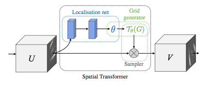
Spatial transformer networks boils down to three main components :

• The localization network is a regular CNN which regresses the transformation parameters. The transformation is never learned explicitly from this dataset, instead the network learns automatically the spatial transformations that enhances the global accuracy.
• The grid generator generates a grid of coordinates in the input image corresponding to each pixel from the output image.
• The sampler uses the parameters of the transformation and applies it to the input image.
• 

• class Net(nn.Module):
      def __init__(self):
          super(Net, self).__init__()
          self.conv1 = nn.Conv2d(1, 10, kernel_size=5)
          self.conv2 = nn.Conv2d(10, 20, kernel_size=5)
          self.conv2_drop = nn.Dropout2d()
          self.fc1 = nn.Linear(320, 50)
          self.fc2 = nn.Linear(50, 10)
  
          # Spatial transformer localization-network
          self.localization = nn.Sequential(
              nn.Conv2d(1, 8, kernel_size=7),
              nn.MaxPool2d(2, stride=2),
              nn.ReLU(True),
              nn.Conv2d(8, 10, kernel_size=5),
              nn.MaxPool2d(2, stride=2),
              nn.ReLU(True)
          )
  
          # Regressor for the 3 * 2 affine matrix
          self.fc_loc = nn.Sequential(
              nn.Linear(10 * 3 * 3, 32),
              nn.ReLU(True),
              nn.Linear(32, 3 * 2)
          )
  
          # Initialize the weights/bias with identity transformation
          self.fc_loc[2].weight.data.zero_()
          self.fc_loc[2].bias.data.copy_(torch.tensor([1, 0, 0, 0, 1, 0], dtype=torch.float))
  
      # Spatial transformer network forward function
      def stn(self, x):
          xs = self.localization(x)
          xs = xs.view(-1, 10 * 3 * 3)
          theta = self.fc_loc(xs)
          theta = theta.view(-1, 2, 3)
  
          grid = F.affine_grid(theta, x.size())
          x = F.grid_sample(x, grid)
  
          return x
  
      def forward(self, x):
          # transform the input
          x = self.stn(x)
  
          # Perform the usual forward pass
          x = F.relu(F.max_pool2d(self.conv1(x), 2))
          x = F.relu(F.max_pool2d(self.conv2_drop(self.conv2(x)), 2))
          x = x.view(-1, 320)
          x = F.relu(self.fc1(x))
          x = F.dropout(x, training=self.training)
          x = self.fc2(x)
          return F.log_softmax(x, dim=1)
  
  
  model = Net().to(device)

  Now, let’s use the SGD algorithm to train the model. The network is learning the classification task in a supervised way. In the same time the model is learning STN automatically in an end-to-end fashion.

• optimizer = optim.SGD(model.parameters(), lr=0.01)
  
  
  def train(epoch):
      model.train()
      for batch_idx, (data, target) in enumerate(train_loader):
          data, target = data.to(device), target.to(device)
  
          optimizer.zero_grad()
          output = model(data)
          loss = F.nll_loss(output, target)
          loss.backward()
          optimizer.step()
          if batch_idx % 500 == 0:
              print('Train Epoch: {} [{}/{} ({:.0f}%)]\tLoss: {:.6f}'.format(
                  epoch, batch_idx * len(data), len(train_loader.dataset),
                  100. * batch_idx / len(train_loader), loss.item()))
  #
  # A simple test procedure to measure the STN performances on MNIST.
  #
  
  
  def test():
      with torch.no_grad():
          model.eval()
          test_loss = 0
          correct = 0
          for data, target in test_loader:
              data, target = data.to(device), target.to(device)
              output = model(data)
  
              # sum up batch loss
              test_loss += F.nll_loss(output, target, reduction='sum').item()
              # get the index of the max log-probability
              pred = output.max(1, keepdim=True)[1]
              correct += pred.eq(target.view_as(pred)).sum().item()
  
          test_loss /= len(test_loader.dataset)
          print('\nTest set: Average loss: {:.4f}, Accuracy: {}/{} ({:.0f}%)\n'
                .format(test_loss, correct, len(test_loader.dataset),
                        100. * correct / len(test_loader.dataset)))

  Now, we will inspect the results of our learned visual attention mechanism.

  We define a small helper function in order to visualize the transformations while training.

• def convert_image_np(inp):
      """Convert a Tensor to numpy image."""
      inp = inp.numpy().transpose((1, 2, 0))
      mean = np.array([0.485, 0.456, 0.406])
      std = np.array([0.229, 0.224, 0.225])
      inp = std * inp + mean
      inp = np.clip(inp, 0, 1)
      return inp
  
  # We want to visualize the output of the spatial transformers layer
  # after the training, we visualize a batch of input images and
  # the corresponding transformed batch using STN.
  
  
  def visualize_stn():
      with torch.no_grad():
          # Get a batch of training data
          data = next(iter(test_loader))[0].to(device)
  
          input_tensor = data.cpu()
          transformed_input_tensor = model.stn(data).cpu()
  
          in_grid = convert_image_np(
              torchvision.utils.make_grid(input_tensor))
  
          out_grid = convert_image_np(
              torchvision.utils.make_grid(transformed_input_tensor))
  
          # Plot the results side-by-side
          f, axarr = plt.subplots(1, 2)
          axarr[0].imshow(in_grid)
          axarr[0].set_title('Dataset Images')
  
          axarr[1].imshow(out_grid)
          axarr[1].set_title('Transformed Images')
  
  for epoch in range(1, 20 + 1):
      train(epoch)
      test()
  
  # Visualize the STN transformation on some input batch
  visualize_stn()
  
  plt.ioff()
  plt.show()