


生成对抗网络
一.GAN(生成式对抗网络)
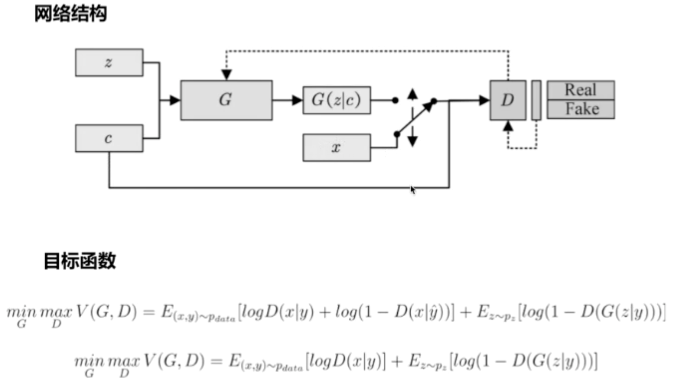
1.基本理论
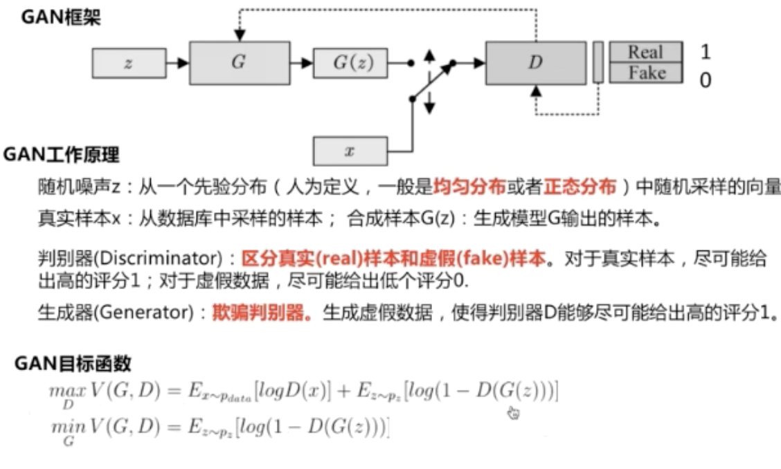
对于目标函数,可以理解为当优化D时,D(x)越大越好,D(G(z))越小越好(能区分真实样本和虚假样本)
当优化G时,D(G(z))越大越好(欺骗判别器)
2.KL散度:
一种衡量两个概率分布的匹配程度的指标
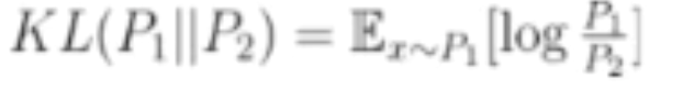
P1=P2时,KL=0
KL散度具有非负性、不对称性
最小化KL散度就可以优化生成对抗网络
3.JS散度:
具有非负性、对称性
![]()
GAN通过对抗训练,间接计算出JS散度
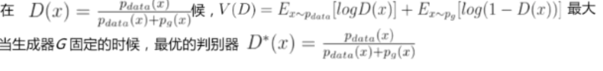
最优判别器大于0小于1,因此用sigmoid激活。


4.代码实现
1).随机初始化生成器和判别器
net_G = nn.Sequential(
            nn.Linear(z_dim,hidden_dim),
            nn.ReLU(),
            nn.Linear(hidden_dim, 2))

# 定义判别器
net_D = nn.Sequential(
            nn.Linear(2,hidden_dim),
            nn.ReLU(),
            nn.Linear(hidden_dim,1),
            nn.Sigmoid())
2).交替训练判别器D和生成器G,直到收敛
a.固定生成器G(不优化),训练判别器D区分真实图像和合成图像(二分类问题)
# 固定生成器G,改进判别器D
        # 使用normal_()函数生成一组随机噪声,输入G得到一组样本
        z = torch.empty(batch_size,z_dim).normal_().to(device)
        fake_batch = net_G(z)
        # 将真、假样本分别输入判别器,得到结果
        D_scores_on_real = net_D(real_batch.to(device))
        D_scores_on_fake = net_D(fake_batch)
        # 优化过程中,假样本的score会越来越小,真样本的score会越来越大,下面 loss 的定义刚好符合这一规律,
        # 要保证loss越来越小,真样本的score前面要加负号
        # 要保证loss越来越小,假样本的score前面是正号(负负得正)
        loss = -torch.mean(torch.log(1-D_scores_on_fake) + torch.log(D_scores_on_real))
        # 梯度清零
        optimizer_D.zero_grad()
        # 反向传播优化
        loss.backward()
        # 更新全部参数
        optimizer_D.step()
        loss_D += loss
b.固定判别器D,训练生成器G欺骗判别器D(最大化问题)
# 固定判别器,改进生成器
        # 生成一组随机噪声,输入生成器得到一组假样本
        z = torch.empty(batch_size,z_dim).normal_().to(device)
        fake_batch = net_G(z)
        # 假样本输入判别器得到 score
        D_scores_on_fake = net_D(fake_batch)
        # 我们希望假样本能够骗过生成器,得到较高的分数,下面的 loss 定义也符合这一规律
        # 要保证 loss 越来越小,假样本的前面要加负号
        loss = -torch.mean(torch.log(D_scores_on_fake))
        optimizer_G.zero_grad()
        loss.backward()
        optimizer_G.step()
        loss_G += loss
关键步骤截图:
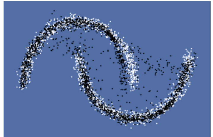
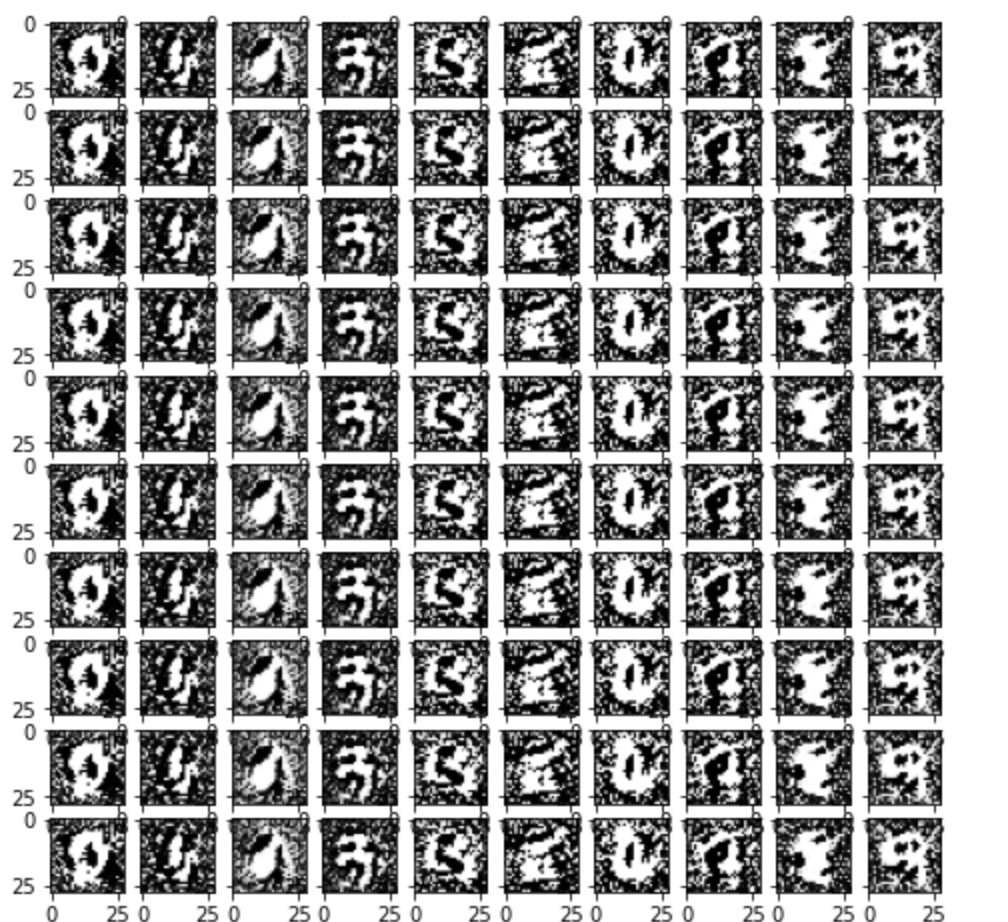
原数据:
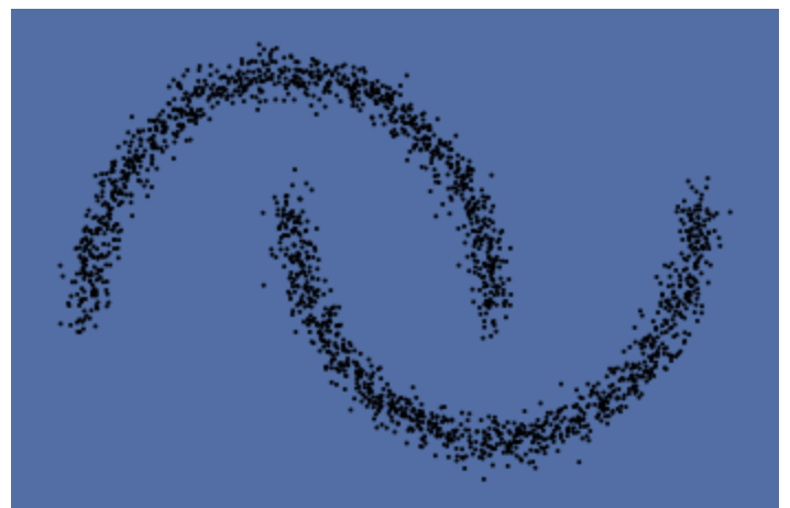
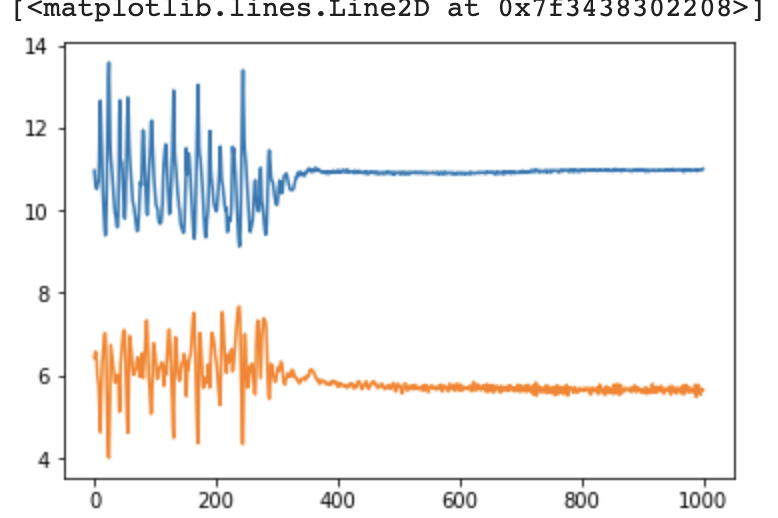
训练loss变换(学习率0.001,batch_size=250)及生成图像:
二.cGAN(条件生成)
1.改进判别器,输入加入标签
2.代码实现:
1)生成器和判别器
class Discriminator(nn.Module):
	'''全连接判别器,用于1x28x28的MNIST数据,输出是数据和类别'''
	def __init__(self):
		super(Discriminator, self).__init__()
		self.model = nn.Sequential(
			  nn.Linear(28*28+10, 512),
			  nn.LeakyReLU(0.2, inplace=True),
			  nn.Linear(512, 256),
			  nn.LeakyReLU(0.2, inplace=True),
			  nn.Linear(256, 1),
			  nn.Sigmoid()
		)

	def forward(self, x, c):
		x = x.view(x.size(0), -1)
		validity = self.model(torch.cat([x, c], -1))
		return validity

class Generator(nn.Module):
	'''全连接生成器,用于1x28x28的MNIST数据,输入是噪声和类别'''
	def __init__(self, z_dim):
		super(Generator, self).__init__()
		self.model = nn.Sequential(
			  nn.Linear(z_dim+10, 128),
			  nn.LeakyReLU(0.2, inplace=True),
			  nn.Linear(128, 256),
			  nn.BatchNorm1d(256, 0.8),
			  nn.LeakyReLU(0.2, inplace=True),
			  nn.Linear(256, 512),
			  nn.BatchNorm1d(512, 0.8),
			  nn.LeakyReLU(0.2, inplace=True),
			  nn.Linear(in_features=512, out_features=28*28),
			  nn.Tanh()
	 	)

	def forward(self, z, c):
		x = self.model(torch.cat([z, c], dim=1))
		x = x.view(-1, 1, 28, 28)
		return x
与GAN唯一的区别是:输入增加了10个维度(0-9)
2)初始化:
for epoch in range(total_epochs):
generator=generator.train()
for i,data in enumerate(dataloader):
real_images,real_labels=data
wrong_labels=[]
for real_label in real_labels:
tmp=np.arange(10).tolist()
tmp.remove(float(real_label.data))
wrong_labels.append(np.random.choice(tmp,1)[0])
wrong_labels=torch.LongTensor(wrong_labels)
real_images=real_images.to(device)
tmp=torch.FloatTensor(real_labels.size(0),10).zero_()
real_labels=tmp.scatter_(dim=1,index=torch.LongTensor(real_labels.view(-1,1)),value=1)
real_labels=real_labels.to(device)
tmp=torch.FloatTensor(real_labels.size(0),10).zero_()
wrong_labels=tmp.scatter_(dim=1,index=torch.LongTensor(wrong_labels.view(-1,1)),value=1)
wrong_labels=wrong_labels.to(device)
z=torch.randn([batch_size,z_dim]).to(device)
c=torch.FloatTensor(batch_size,10).zero_()
c=c.scatter_(dim=1,index=torch.LongTensor(np.random.choice(10,batch_size).reshape([batch_size,1])),value=1)
c=c.to(device)
fake_images=generator(z,c)
real_loss=bce(discriminator(real_images,real_labels).squeeze(-1),ones)
fake_loss_1=bce(discriminator(fake_images.detach(),c).squeeze(-1),zeros)
fake_loss_2=bce(discriminator(real_images,wrong_labels).squeeze(-1),zeros)
d_loss=real_loss+fake_loss_1+fake_loss_2
d_optimizer.zero_grad()
d_loss.backward()
d_optimizer.step()
g_loss=bce(discriminator(fake_images,c).squeeze(-1),ones)
g_optimizer.zero_grad()
g_loss.backward()
g_optimizer.step()
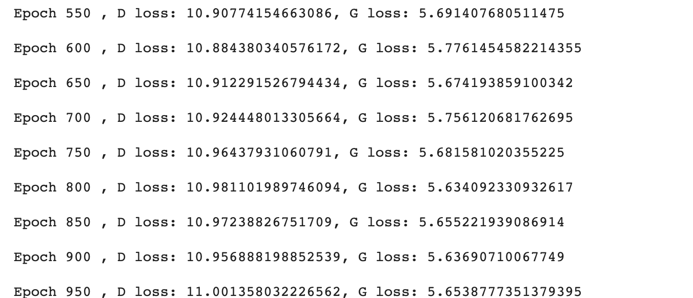
print("[Epoch %d/%d] [D loss: %f] [G loss: %f]" % (epoch, total_epochs, d_loss.item(), g_loss.item()))
比较值得注意的是loss的计算,可以概括为 正确的图像和正确的标签(1)+正确的图像和错误的标签(0)+错误的图像(0)
3)结果显示
效果比较差,尝试了修改部分参数、加入wrong_label判别以及增加训练轮数,但对结果都没有太大改善。
三.DCGAN
1.区别:
前两个都是使用全连接神经网络,DCGAN是卷积神经网络(偏向实验和工程)
2.判别器和生成器:
判别器使用滑动卷积(step>1),不用pooling
生成器使用滑动反卷积
3.使用批归一化
4.激活函数使用Relu( )或PRelu( )
5.代码实现
1)判别器和生成器
判别器
	'''滑动卷积判别器'''
	def __init__(self):
		super(D_dcgan, self).__init__()
		self.conv = nn.Sequential(
            # 第一个滑动卷积层,不使用BN,LRelu激活函数
            nn.Conv2d(in_channels=1, out_channels=16, kernel_size=3, stride=2, padding=1),
            nn.LeakyReLU(0.2, inplace=True),
            # 第二个滑动卷积层,包含BN,LRelu激活函数
            nn.Conv2d(in_channels=16, out_channels=32, kernel_size=3, stride=2, padding=1),
            nn.BatchNorm2d(32),
            nn.LeakyReLU(0.2, inplace=True),
            # 第三个滑动卷积层,包含BN,LRelu激活函数
            nn.Conv2d(in_channels=32, out_channels=64, kernel_size=3, stride=2, padding=1),
            nn.BatchNorm2d(64),
            nn.LeakyReLU(0.2, inplace=True),
            # 第四个滑动卷积层,包含BN,LRelu激活函数
            nn.Conv2d(in_channels=64, out_channels=128, kernel_size=4, stride=1),
            nn.BatchNorm2d(128),
            nn.LeakyReLU(0.2, inplace=True)
        )

		# 全连接层+Sigmoid激活函数
		self.linear = nn.Sequential(nn.Linear(in_features=128, out_features=1), nn.Sigmoid())

	def forward(self, x):
		x = self.conv(x)
		x = x.view(x.size(0), -1)
		validity = self.linear(x)
		return validity
生成器
class G_dcgan(nn.Module):
	'''反滑动卷积生成器'''

	def __init__(self, z_dim):
		super(G_dcgan, self).__init__()
		self.z_dim = z_dim
		# 第一层:把输入线性变换成256x4x4的矩阵,并在这个基础上做反卷机操作
		self.linear = nn.Linear(self.z_dim, 4*4*256)
		self.model = nn.Sequential(
            # 第二层:bn+relu
            nn.ConvTranspose2d(in_channels=256, out_channels=128, kernel_size=3, stride=2, padding=0),
            nn.BatchNorm2d(128),
            nn.ReLU(inplace=True),
            # 第三层:bn+relu
            nn.ConvTranspose2d(in_channels=128, out_channels=64, kernel_size=3, stride=2, padding=1),
            nn.BatchNorm2d(64),
            nn.ReLU(inplace=True),
            # 第四层:不使用BN,使用tanh激活函数
            nn.ConvTranspose2d(in_channels=64, out_channels=1, kernel_size=4, stride=2, padding=2),
            nn.Tanh()
        )

	def forward(self, z):
		# 把随机噪声经过线性变换,resize成256x4x4的大小
		x = self.linear(z)
		x = x.view([x.size(0), 256, 4, 4])
		# 生成图片
		x = self.model(x)
		return x
2)训练结果

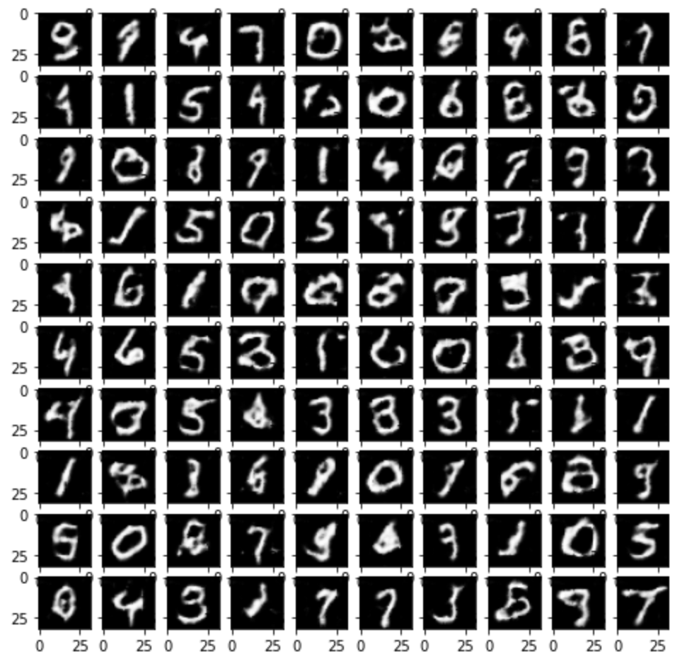
发现训练结果明显好于以上两个网络。

 浙公网安备 33010602011771号