(六) 6.3 Neurons Networks Gradient Checking
BP算法很难调试,一般情况下会隐隐存在一些小问题,比如(off-by-one error),即只有部分层的权重得到训练,或者忘记计算bais unit,这虽然会得到一个正确的结果,但效果差于准确BP得到的结果。
有了cost function,目标是求出一组参数W,b,这里以 表示,cost function 暂且记做
 。假设
。假设  ,则
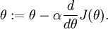
,则  ,即一维情况下的Gradient Descent:
根据6.2中对单个参数单个样本的求导公式:
可以得到每个参数的偏导数,对所有样本累计求和,可以得到所有训练数据对参数 的偏导数记做  , 是靠BP算法求得的,为了验证其正确性,看下图回忆导数公式:
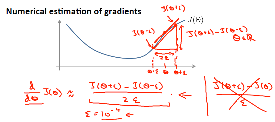
可见有: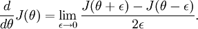 那么对于任意 值,我们都可以对等式左边的导数用:
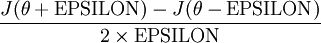 来近似。
来近似。
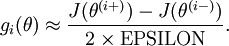
给定一个被认为能计算  的函数,可以用下面的数值检验公式
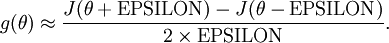
应用时,通常把 设置为一个很小的常量,比如在
 数量级,最好不要太小了,会造成数值的舍入误差。上式两端值的接近程度取决于
  的具体形式。假定
 的情况下,上式左右两端至少有4位有效数字是一样的(通常会更多)。
当 是一个n维向量而不是实数时,且
  ,在 Neorons Network 中,J(W,b)可以想象为 W,b 组合扩展而成的一个长向量 ,现在又一个计算
  的函数
的函数  ,如何检验能否输出到正确结果呢,用的取值来检验,对于向量的偏导数:
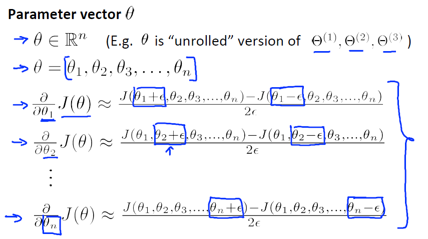
根据上图,对 i 求导时,只需要在向量的第i维上进行加减操作,然后求值即可,定义  ,其中
,其中
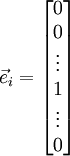
 和 几乎相同,除了第
  行元素增加了 ,类似地,
 得到的第 行减小了 ,然后求导并与比较:
 中的参数对应的是参数向量中一个分量的细微变化,损失函数J 在不同情况下会有不同的值(比如三层NN 或者 三层autoencoder(需加上稀疏项)),上式中左边为BP算法的结果,右边为真正的梯度,只要两者很接近,说明BP算法是在正确工作,对于梯度下降中的参数是按照如下方式进行更新的:
![\begin{align}
W^{(l)} &= W^{(l)} - \alpha \left[ \left(\frac{1}{m} \Delta W^{(l)} \right) + \lambda W^{(l)}\right] \\
b^{(l)} &= b^{(l)} - \alpha \left[\frac{1}{m} \Delta b^{(l)}\right]
\end{align}](http://ufldl.stanford.edu/wiki/images/math/0/f/7/0f7430e97ec4df1bfc56357d1485405f.png)
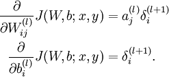
即有 分别为:
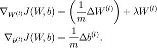
最后只需总体损失函数J(W,b)的偏导数与上述 的值比较即可。
除了梯度下降外,其他的常见的优化算法:1) 自适应 的步长,2) BFGS L-BFGS,3) SGD,4) 共轭梯度算法,以后涉及到再看。

 浙公网安备 33010602011771号