MATLAB 颜色图函数(imagesc/scatter/polarPcolor/pcolor)
2维的热度图 imagesc
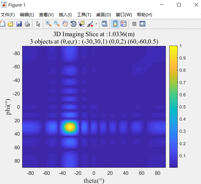
imagesc(x, y, z),x和y分别是横纵坐标,z为值,表示颜色
imagesc(theta,phi,slc); colorbar
xlabel('theta(°)','fontname','Times New Roman','FontSize',14);
ylabel('phi(°)','fontname','Times New Roman','FontSize',14);
sta = '3 objects at (θ,φ,r) : (-30,30,1) (0,0,2) (60,-60,0.5)';
str=sprintf(strcat('3D Imaging Slice at :', num2str(d_max*D/N), '(m)', '\n',sta));
title(str, 'fontname','Times New Roman','Color','k','FontSize',13);
grid on
其中,colorbar的坐标值调整:caxis([0 1]);
colormap的色系调整:colormap hot
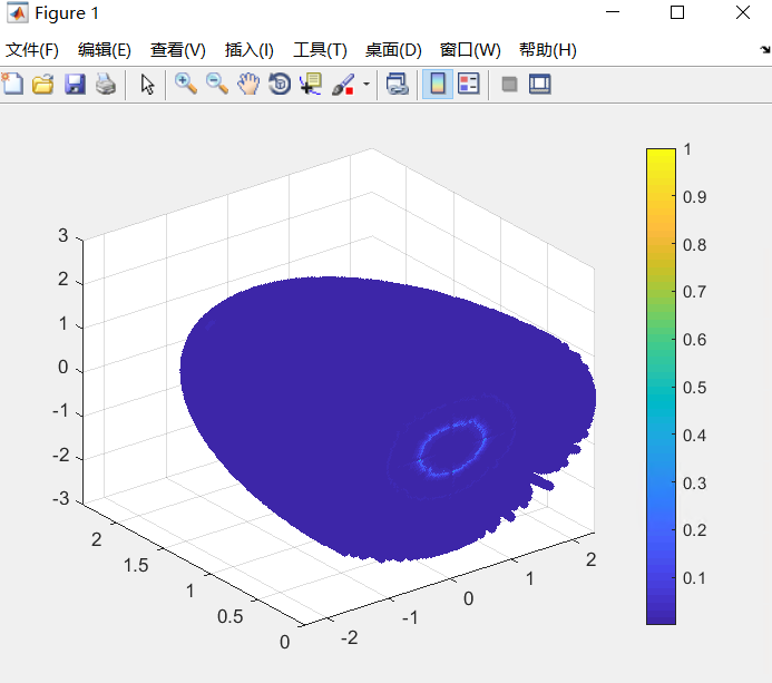
3维散点图 scatter
scatter3(x,y,z,24,c,'filled');
% axis([-(R+2) (R+2) -(R+2) (R+2) 0 (h+2)]);
colorbar
2维 极坐标热度图 polarPcolor
polarPcolor(R_axis, theta, value),前两个为半径方向坐标轴和圆心角坐标轴,value为值,用颜色表示
[fig, clr] = polarPcolor(R_axis, theta, x_d_th, 'labelR','range (m)','Ncircles', 5,'Nspokes',7);
colormap hot
% caxis([0 1]);

其中polarPcolor代码如下:
function [varargout] = polarPcolor(R,theta,Z,varargin)
% [h,c] = polarPcolor1(R,theta,Z,varargin) is a pseudocolor plot of matrix
% Z for a vector radius R and a vector angle theta.
% The elements of Z specify the color in each cell of the
% plot. The goal is to apply pcolor function with a polar grid, which
% provides a better visualization than a cartesian grid.
%
%% Syntax
%
% [h,c] = polarPcolor(R,theta,Z)
% [h,c] = polarPcolor(R,theta,Z,'Ncircles',10)
% [h,c] = polarPcolor(R,theta,Z,'Nspokes',5)
% [h,c] = polarPcolor(R,theta,Z,'Nspokes',5,'colBar',0)
% [h,c] = polarPcolor(R,theta,Z,'Nspokes',5,'labelR','r (km)')
%
% INPUT
%    * R :
%        - type: float
%        - size: [1 x Nrr ] where Nrr = numel(R).
%        - dimension: radial distance.
%    * theta :
%        - type: float
%        - size: [1 x Ntheta ] where Ntheta = numel(theta).
%        - dimension: azimuth or elevation angle (deg).
%        - N.B.: The zero is defined with respect to the North.
%    * Z :
%        - type: float
%        - size: [Ntheta x Nrr]
%        - dimension: user's defined .
%    * varargin:
%        - Ncircles: number  of circles for the grid definition.
%        - Nspokes: number of spokes for the grid definition.
%        - colBar: display the colorbar or not.
%        - labelR: legend for R.
%
%
% OUTPUT
% h: returns a handle to a SURFACE object.
% c: returns a handle to a COLORBAR object.
%
%% Examples
% R = linspace(3,10,100);
% theta = linspace(0,180,360);
% Z = linspace(0,10,360)'*linspace(0,10,100);
% figure
% polarPcolor(R,theta,Z,'Ncircles',3)
%
%% Author
% Etienne Cheynet, University of Stavanger, Norway. 28/05/2016
% see also pcolor
%

%%  InputParseer
p = inputParser();
p.CaseSensitive = false;
p.addOptional('Ncircles',5);
p.addOptional('Nspokes',8);
p.addOptional('labelR','');
p.addOptional('colBar',1);
p.parse(varargin{:});

Ncircles = p.Results.Ncircles ;
Nspokes = p.Results.Nspokes ;
labelR = p.Results.labelR ;
colBar = p.Results.colBar ;
%% Preliminary checks
% case where dimension is reversed
Nrr = numel(R);
Noo = numel(theta);
if isequal(size(Z),[Noo,Nrr]),
    Z=Z';
end

% case where dimension of Z is not compatible with theta and R
if ~isequal(size(Z),[Nrr,Noo])
    fprintf('\n')
    fprintf([ 'Size of Z is : [',num2str(size(Z)),'] \n']);
    fprintf([ 'Size of R is : [',num2str(size(R)),'] \n']);
    fprintf([ 'Size of theta is : [',num2str(size(theta)),'] \n\n']);
    error(' dimension of Z does not agree with dimension of R and Theta')
end
%% data plot
rMin = min(R);
rMax = max(R);
thetaMin=min(theta);
thetaMax =max(theta);
% Definition of the mesh
Rrange = rMax - rMin; % get the range for the radius
rNorm = R/Rrange; %normalized radius [0,1]
% get hold state
cax = newplot;
% transform data in polar coordinates to Cartesian coordinates.
YY = (rNorm)'*cosd(theta);
XX = (rNorm)'*sind(theta);
% plot data on top of grid
h = pcolor(XX,YY,Z,'parent',cax);
shading flat
set(cax,'dataaspectratio',[1 1 1]);axis off;
if ~ishold(cax);
    % make a radial grid
    hold(cax,'on')
    % Draw circles and spokes
    createSpokes(thetaMin,thetaMax,Ncircles,Nspokes);
    createCircles(rMin,rMax,thetaMin,thetaMax,Ncircles,Nspokes)
end

%% PLot colorbar if specified
if colBar==1,
    c =colorbar('location','WestOutside');
    caxis([quantile(Z(:),0.01),quantile(Z(:),0.99)])
else
    c = [];
end

%% Outputs
nargoutchk(0,2)
if nargout==1,
    varargout{1}=h;
elseif nargout==2,
    varargout{1}=h;
    varargout{2}=c;
end

%%%%%%%%%%%%%%%%%%%%%%%%%%%%%%%%%%%%%%%%%%%%%%%%%%%%%%%%%%%%%%%%%%%%%%%%%%%
% Nested functions
%%%%%%%%%%%%%%%%%%%%%%%%%%%%%%%%%%%%%%%%%%%%%%%%%%%%%%%%%%%%%%%%%%%%%%%%%%%
    function createSpokes(thetaMin,thetaMax,Ncircles,Nspokes)

        circleMesh = linspace(rMin,rMax,Ncircles);
        spokeMesh = linspace(thetaMin,thetaMax,Nspokes);
        contour = abs((circleMesh - circleMesh(1))/Rrange+R(1)/Rrange);
        cost = cosd(90-spokeMesh); % the zero angle is aligned with North
        sint = sind(90-spokeMesh); % the zero angle is aligned with North
        for kk = 1:Nspokes
            plot(cost(kk)*contour,sint(kk)*contour,'k:',...
                'handlevisibility','off');
            % plot graduations of angles
            % avoid superimposition of 0 and 360
            if and(thetaMin==0,thetaMax == 360),
                if spokeMesh(kk)<360,

                    text(1.05.*contour(end).*cost(kk),...
                        1.05.*contour(end).*sint(kk),...
                        [num2str(spokeMesh(kk),3),char(176)],...
                        'horiz', 'center', 'vert', 'middle');
                end
            else
                text(1.05.*contour(end).*cost(kk),...
                    1.05.*contour(end).*sint(kk),...
                    [num2str(spokeMesh(kk),3),char(176)],...
                    'horiz', 'center', 'vert', 'middle');
            end

        end
    end
    function createCircles(rMin,rMax,thetaMin,thetaMax,Ncircles,Nspokes)

        % define the grid in polar coordinates
        angleGrid = linspace(90-thetaMin,90-thetaMax,100);
        xGrid = cosd(angleGrid);
        yGrid = sind(angleGrid);
        circleMesh = linspace(rMin,rMax,Ncircles);
        spokeMesh = linspace(thetaMin,thetaMax,Nspokes);
        contour = abs((circleMesh - circleMesh(1))/Rrange+R(1)/Rrange);
        % plot circles
        for kk=1:length(contour)
            plot(xGrid*contour(kk), yGrid*contour(kk),'k:');
        end
        % radius tick label
        for kk=1:Ncircles

            position = 0.51.*(spokeMesh(min(Nspokes,round(Ncircles/2)))+...
                spokeMesh(min(Nspokes,1+round(Ncircles/2))));

            if abs(round(position)) ==90,
                % radial graduations
                text((contour(kk)).*cosd(90-position),...
                    (0.1+contour(kk)).*sind(86-position),...
                    num2str(circleMesh(kk),2),'verticalalignment','BaseLine',...
                    'horizontalAlignment', 'center',...
                    'handlevisibility','off','parent',cax);

                % annotate spokes
                text(contour(end).*0.6.*cosd(90-position),...
                    0.07+contour(end).*0.6.*sind(90-position),...
                    [labelR],'verticalalignment','bottom',...
                    'horizontalAlignment', 'right',...
                    'handlevisibility','off','parent',cax);
            else
                % radial graduations
                text((contour(kk)).*cosd(90-position),...
                    (contour(kk)).*sind(90-position),...
                    num2str(circleMesh(kk),2),'verticalalignment','BaseLine',...
                    'horizontalAlignment', 'right',...
                    'handlevisibility','off','parent',cax);

                % annotate spokes
                text(contour(end).*0.6.*cosd(90-position),...
                    contour(end).*0.6.*sind(90-position),...
                    [labelR],'verticalalignment','bottom',...
                    'horizontalAlignment', 'right',...
                    'handlevisibility','off','parent',cax);
            end
        end

    end
end
再贴一个示例代码:
%% Examples
% The following examples illustrate the application of the function
% polarPcolor
clearvars;close all;clc;

%% Minimalist example
% Assuming that a remote sensor is measuring the wind field for a radial
% distance ranging from 50 to 1000 m. The scanning azimuth is oriented from
% North (0 deg) to North-North-East ( 80 deg):
R = linspace(50,1000,100)./1000; % (distance in km)
Az = linspace(0,80,100); % in degrees
[~,~,windSpeed] = peaks(100); % radial wind speed
figure(1)
[h,c]=polarPcolor(R,Az,windSpeed);

%% Example with options
%  We want to have 4 circles and 7 spokes, and to give a label to the
%  radial coordinate

figure(2)
[~,c]=polarPcolor(R,Az,windSpeed,'labelR','r (km)','Ncircles',7,'Nspokes',7);
ylabel(c,' radial wind speed (m/s)');
set(gcf,'color','w')
%% Dealing with outliers
% We introduce outliers in the wind velocity data. These outliers
% are represented as wind speed sample with a value of 100 m/s. These
% corresponds to unrealistic data that need to be ignored. To avoid bad
% scaling of the colorbar, the function polarPcolor uses the function caxis
% combined to the function quantile to keep the colorbar properly scaled:
% caxis([quantile(Z(:),0.01),quantile(Z(:),0.99)])

windSpeed(1:10:end,1:20:end)=100;

figure(3)
[~,c]=polarPcolor(R,Az,windSpeed);
ylabel(c,' radial wind speed (m/s)');
set(gcf,'color','w')

%% polarPcolor without colorbar
% The colorbar is activated by default. It is possible to remove it by
% using the option 'colBar'. When the colorbar is desactivated, the
% outliers are not "removed" and bad scaling is clearly visible:

figure(4)
polarPcolor(R,Az,windSpeed,'colBar',0) ;


%% Different geometry 1
N = 360;
R = linspace(0,1000,N)./1000; % (distance in km)
Az = linspace(0,360,N); % in degrees
[~,~,windSpeed] = peaks(N); % radial wind speed
figure(5)
[~,c]= polarPcolor(R,Az,windSpeed);
ylabel(c,' radial wind speed (m/s)');
set(gcf,'color','w')
%% Different geometry 2
N = 360;
R = linspace(500,1000,N)./1000; % (distance in km)
Az = linspace(0,270,N); % in degrees
[~,~,windSpeed] = peaks(N); % radial wind speed
figure(6)
[~,c]= polarPcolor(R,Az,windSpeed,'Ncircles',3);
location = 'NorthOutside';
ylabel(c,' radial wind speed (m/s)');
set(c,'location',location);
set(gcf,'color','w')

 浙公网安备 33010602011771号