SuperPoint
 提出了一种全卷积神经网络架构,用于兴趣点检测和描述,该架构使用一种名为单应性自适应(Homographic Adaptation)的自监督域自适应框架进行训练。我们的实验表明:(1)可以将知识从合成数据集迁移到真实世界的图像上;(2)稀疏兴趣点检测和描述可以作为一个高效的卷积神经网络来实现;(3)由此产生的系统在诸如单应性估计等几何计算机视觉匹配任务中表现良好。
| 英文题目 | SuperPoint: Self-Supervised Interest Point Detection and Description |
|---|---|
| 中文名称 | SuperPoint:自监督兴趣点检测与描述 |
| 发表时间 | 2017年12月20日 |
| 平台 | CVPR 2018 |
| 作者 | Daniel DeTone, Tomasz Malisiewicz, Andrew Rabinovich |
| 邮箱 | {ddetone, tmalisiewicz, arabinovich}@magicleap.com |
| 来源 | Magic Leap Sunnyvale, CA |
| 关键词 | 关键点提取 |
| paper && code && video | paper code video |
Abstract
摘要
This paper presents a self-supervised framework for training interest point detectors and descriptors suitable for a large number of multiple-view geometry problems in computer vision. As opposed to patch-based neural networks, our fully-convolutional model operates on full-sized images and jointly computes pixel-level interest point locations and associated descriptors in one forward pass. We introduce Homographic Adaptation, a multi-scale, multi-homography approach for boosting interest point detection repeatability and performing cross-domain adaptation (e.g., synthetic-to-real). Our model, when trained on the MS-COCO generic image dataset using Homographic Adaptation, is able to repeatedly detect a much richer set of interest points than the initial pre-adapted deep model and any other traditional corner detector. The final system gives rise to state-of-the-art homography estimation results on HPatches when compared to LIFT, SIFT and ORB.
本文提出了一个自监督框架,用于训练适用于计算机视觉中大量多视图几何问题的兴趣点检测器和描述符。与基于图像块的神经网络不同,我们的全卷积模型可处理全尺寸图像,并在一次前向传播中联合计算像素级兴趣点位置和相关描述符。我们引入了单应性自适应(Homographic Adaptation)方法,这是一种多尺度、多单应性的方法,用于提高兴趣点检测的重复性并进行跨领域自适应(例如,从合成数据到真实数据)。当使用单应性自适应方法在MS - COCO通用图像数据集上训练我们的模型时,与初始预自适应的深度模型以及其他任何传统角点检测器相比,它能够重复检测到更丰富的兴趣点集。与LIFT、SIFT和ORB相比,最终系统在HPatches数据集上实现了最先进的单应性估计结果。
1. Introduction
1. 引言
The first step in geometric computer vision tasks such as Simultaneous Localization and Mapping (SLAM), Structure-from-Motion (SfM), camera calibration, and image matching is to extract interest points from images. Interest points are 2D locations in an image which are stable and repeatable from different lighting conditions and viewpoints. The subfield of mathematics and computer vision known as Multiple View Geometry [9] consists of theorems and algorithms built on the assumption that interest points can be reliably extracted and matched across images. However, the inputs to most real-world computer vision systems are raw images, not idealized point locations.
在诸如同步定位与地图构建(Simultaneous Localization and Mapping,SLAM)、运动恢复结构(Structure - from - Motion,SfM)、相机校准和图像匹配等几何计算机视觉任务中,第一步是从图像中提取兴趣点。兴趣点是图像中的二维位置,在不同光照条件和视角下具有稳定性和重复性。数学和计算机视觉的一个子领域——多视图几何[9],包含了基于兴趣点能够在不同图像中可靠提取和匹配这一假设构建的定理和算法。然而,大多数现实世界计算机视觉系统的输入是原始图像,而非理想化的点位置。
Convolutional neural networks have been shown to be superior to hand-engineered representations on almost all tasks requiring images as input. In particular, fully-convolutional neural networks which predict 2D "key-points" or "landmarks" are well-studied for a variety of tasks such as human pose estimation [31], object detection [14], and room layout estimation [12]. At the heart of these techniques is a large dataset of \(2\mathrm{D}\) ground truth locations labeled by human annotators.
卷积神经网络在几乎所有需要图像作为输入的任务中都表现出优于手工设计表示的性能。特别是,用于预测二维“关键点”或“地标”的全卷积神经网络在诸如人体姿态估计[31]、目标检测[14]和房间布局估计[12]等各种任务中得到了深入研究。这些技术的核心是一个由人工标注的\(2\mathrm{D}\)真实位置的大型数据集。

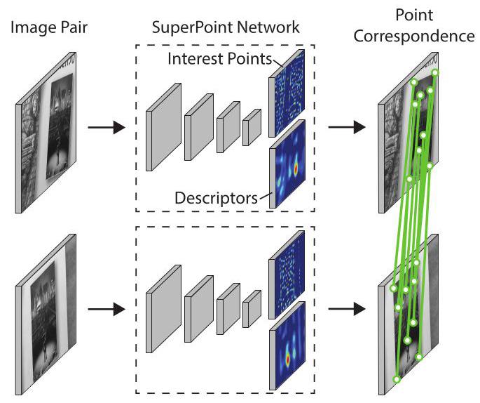
Figure 1. SuperPoint for Geometric Correspondences. We present a fully-convolutional neural network that computes SIFT-like 2D interest point locations and descriptors in a single forward pass and runs at 70 FPS on \({480} \times {640}\) images with a Titan X GPU.
图1. 用于几何对应关系的SuperPoint。我们提出了一种全卷积神经网络,它可以在一次前向传播中计算类似SIFT的二维兴趣点位置和描述符,并且在配备Titan X GPU的情况下,对\({480} \times {640}\)图像的处理速度可达70帧每秒。
It seems natural to similarly formulate interest point detection as a large-scale supervised machine learning problem and train the latest convolutional neural network architecture to detect them. Unfortunately, when compared to semantic tasks such as human-body keypoint estimation, where a network is trained to detect body parts such as the corner of the mouth or left ankle, the notion of interest point detection is semantically ill-defined. Thus training convolution neural networks with strong supervision of interest points is non-trivial.
同样地,将兴趣点检测表述为一个大规模有监督的机器学习问题,并训练最新的卷积神经网络架构来检测它们,这似乎是很自然的。不幸的是,与人体关键点估计等语义任务相比(在人体关键点估计中,网络被训练来检测诸如嘴角或左脚踝等身体部位),兴趣点检测的概念在语义上定义不明确。因此,在兴趣点的强监督下训练卷积神经网络并非易事。
Instead of using human supervision to define interest points in real images, we present a self-supervised solution using self-training. In our approach, we create a large dataset of pseudo-ground truth interest point locations in real images, supervised by the interest point detector itself, rather than a large-scale human annotation effort.
我们没有使用人工监督来定义真实图像中的兴趣点,而是提出了一种使用自训练的自监督解决方案。在我们的方法中,我们创建了一个包含真实图像中伪真实兴趣点位置的大型数据集,该数据集由兴趣点检测器本身监督,而不是通过大规模的人工标注工作。
To generate the pseudo-ground truth interest points, we first train a fully-convolutional neural network on millions of examples from a synthetic dataset we created called Synthetic Shapes (see Figure 2a). The synthetic dataset consists of simple geometric shapes with no ambiguity in the interest point locations. We call the resulting trained detector MagicPoint-it significantly outperforms traditional interest point detectors on the synthetic dataset (see Section 4). MagicPoint performs surprising well on real images despite domain adaptation difficulties [7]. However, when compared to classical interest point detectors on a diverse set of image textures and patterns, MagicPoint misses many potential interest point locations. To bridge this gap in performance on real images, we developed a multi-scale, multi-transform technique - Homographic Adaptation.
为了生成伪真实兴趣点,我们首先在我们创建的一个名为“合成形状”(Synthetic Shapes,见图2a)的合成数据集的数百万个示例上训练一个全卷积神经网络。该合成数据集由简单的几何形状组成,兴趣点位置明确。我们将训练得到的检测器称为MagicPoint——在合成数据集上,它的性能明显优于传统的兴趣点检测器(见第4节)。尽管存在领域适应困难[7],但MagicPoint在真实图像上的表现也出奇地好。然而,与经典的兴趣点检测器在各种图像纹理和图案上进行比较时,MagicPoint会错过许多潜在的兴趣点位置。为了弥补在真实图像上的性能差距,我们开发了一种多尺度、多变换技术——单应性自适应(Homographic Adaptation)。
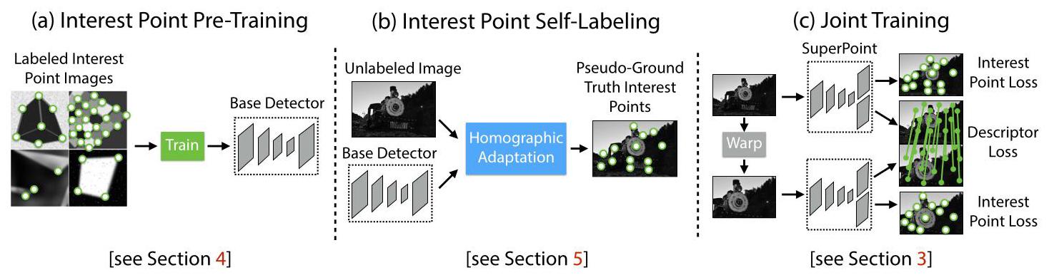
Figure 2. Self-Supervised Training Overview. In our self-supervised approach, we (a) pre-train an initial interest point detector on synthetic data and (b) apply a novel Homographic Adaptation procedure to automatically label images from a target, unlabeled domain. The generated labels are used to (c) train a fully-convolutional network that jointly extracts interest points and descriptors from an image.
图2. 自监督训练概述。在我们的自监督方法中,我们(a)在合成数据上预训练一个初始的兴趣点检测器,(b)应用一种新颖的单应性自适应程序来自动标记来自目标未标记领域的图像。生成的标签用于(c)训练一个全卷积网络,该网络可以从图像中联合提取兴趣点和描述符。
Homographic Adaptation is designed to enable self-supervised training of interest point detectors. It warps the input image multiple times to help an interest point detector see the scene from many different viewpoints and scales (see Section 5). We use Homographic Adaptation in conjunction with the MagicPoint detector to boost the performance of the detector and generate the pseudo-ground truth interest points (see Figure 2b). The resulting detections are more repeatable and fire on a larger set of stimuli; thus we named the resulting detector SuperPoint.
单应性自适应旨在实现兴趣点检测器的自监督训练。它会多次对输入图像进行变换,以帮助兴趣点检测器从多个不同的视角和尺度观察场景(见第5节)。我们将单应性自适应与MagicPoint检测器结合使用,以提高检测器的性能并生成伪真实兴趣点(见图2b)。得到的检测结果更具重复性,并且能对更多的刺激做出响应;因此,我们将得到的检测器命名为SuperPoint。
The most common step after detecting robust and repeatable interest points is to attach a fixed dimensional descriptor vector to each point for higher level semantic tasks, e.g., image matching. Thus we lastly combine SuperPoint with a descriptor subnetwork (see Figure 2c). Since the Super-Point architecture consists of a deep stack of convolutional layers which extract multi-scale features, it is straightforward to then combine the interest point network with an additional subnetwork that computes interest point descriptors (see Section 3). The resulting system is shown in Figure 1.
在检测到稳健且可重复的兴趣点之后,最常见的步骤是为每个点附加一个固定维度的描述符向量,以用于更高级别的语义任务,例如图像匹配。因此,我们最后将SuperPoint与一个描述符子网络相结合(见图2c)。由于SuperPoint架构由深度堆叠的卷积层组成,这些卷积层可以提取多尺度特征,因此将兴趣点网络与一个额外的计算兴趣点描述符的子网络相结合是很直接的(见第3节)。最终的系统如图1所示。
2. Related Work
2. 相关工作
Traditional interest point detectors have been thoroughly evaluated \(\left\lbrack {{24},{16}}\right\rbrack\) . The FAST corner detector [21] was the first system to cast high-speed corner detection as a machine learning problem, and the Scale-Invariant Feature Transform, or SIFT [15], is still probably the most well-known traditional local feature descriptor in computer vision.
传统的兴趣点检测器已经得到了全面的评估 \(\left\lbrack {{24},{16}}\right\rbrack\) 。FAST角点检测器[21]是第一个将高速角点检测作为机器学习问题的系统,而尺度不变特征变换(Scale-Invariant Feature Transform,SIFT)[15]可能仍然是计算机视觉中最著名的传统局部特征描述符。
Our SuperPoint architecture is inspired by recent advances in applying deep learning to interest point detection and descriptor learning. At the ability to match image substructures, we are similar to UCN [3] and to a lesser extent DeepDesc [6]; however, both do not perform any interest point detection. On the other end, LIFT [32], a recently introduced convolutional replacement for SIFT stays close to the traditional patch-based detect then describe recipe. The LIFT pipeline contains interest point detection, orientation estimation and descriptor computation, but additionally requires supervision from a classical SfM system. These differences are summarized in Table 1.
我们的SuperPoint架构受到了最近将深度学习应用于兴趣点检测和描述符学习的进展的启发。在匹配图像子结构的能力方面,我们与UCN[3]类似,在一定程度上也与DeepDesc[6]类似;然而,这两者都不进行任何兴趣点检测。另一方面,LIFT[32]是最近提出的一种替代SIFT的卷积方法,它与传统的基于图像块的先检测后描述的方法相近。LIFT流程包括兴趣点检测、方向估计和描述符计算,但还需要经典的结构从运动(Structure from Motion,SfM)系统的监督。这些差异总结在表1中。
| Interest Points? | Descriptors? | Full Image Input? | Single Network? | Real Time? | |
| SuperPoint (ours) | ✓ | ✓ | ✓ | ✓ | ✓ |
| LIFT [32] | ✓ | ✓ | |||
| UCN [3] | ✓ | ✓ | ✓ | ||
| TILDE [29] | ✓ | ✓ | |||
| DeepDesc [6] | ✓ | ✓ | |||
| SIFT | ✓ | ✓ | |||
| ORB | ✓ | ✓ | ✓ |
Table 1. Qualitative Comparison to Relevant Methods. Our Su-perPoint method is the only one to compute both interest points and descriptors in a single network in real-time.
表1. 与相关方法的定性比较。我们的SuperPoint方法是唯一一种能够在单个网络中实时计算兴趣点和描述符的方法。
On the other extreme of the supervision spectrum, Quad-Networks [23] tackles the interest point detection problem from an unsupervised approach; however, their system is patch-based (inputs are small image patches) and relatively shallow 2-layer network. The TILDE [29] interest point detection system used a principle similar to Homographic Adaptation; however, their approach does not benefit from the power of large fully-convolutional neural networks.
在监督范围的另一个极端,Quad-Networks[23]从无监督的方法来解决兴趣点检测问题;然而,它们的系统是基于图像块的(输入是小图像块),并且是相对较浅的两层网络。TILDE[29]兴趣点检测系统使用了类似于单应性自适应的原理;然而,它们的方法没有受益于大型全卷积神经网络的强大能力。
Our approach can also be compared to other self-supervised methods, synthetic-to-real domain-adaptation methods. A similar approach to Homographic Adaptation is by Honari et al. [10] under the name "equivariant landmark transform." Also, Geometric Matching Networks [20] and Deep Image Homography Estimation [4] use a similar self-supervision strategy to create training data for estimating global transformations. However, these methods lack interest points and point correspondences, which are typically required for doing higher level computer vision tasks such as SLAM and SfM. Joint pose and depth estimation models also exist \(\left\lbrack {{33},{30},{28}}\right\rbrack\) , but do not use interest points.
我们的方法也可以与其他自监督方法、从合成到真实的领域自适应方法进行比较。与单应性自适应(Homographic Adaptation)类似的方法是霍纳里(Honari)等人 [10] 提出的名为“等变地标变换(equivariant landmark transform)”的方法。此外,几何匹配网络(Geometric Matching Networks) [20] 和深度图像单应性估计(Deep Image Homography Estimation) [4] 使用了类似的自监督策略来创建用于估计全局变换的训练数据。然而,这些方法缺乏兴趣点和点对应关系,而这些通常是进行诸如同时定位与地图构建(SLAM)和运动结构恢复(SfM)等更高级计算机视觉任务所必需的。联合姿态和深度估计模型也存在 \(\left\lbrack {{33},{30},{28}}\right\rbrack\) ,但不使用兴趣点。
3. SuperPoint Architecture
3. SuperPoint架构
We designed a fully-convolutional neural network architecture called SuperPoint which operates on a full-sized image and produces interest point detections accompanied by fixed length descriptors in a single forward pass (see Figure 3). The model has a single, shared encoder to process and reduce the input image dimensionality. After the encoder, the architecture splits into two decoder "heads", which learn task specific weights - one for interest point detection and the other for interest point description. Most of the network's parameters are shared between the two tasks, which is a departure from traditional systems which first detect interest points, then compute descriptors and lack the ability to share computation and representation across the two tasks.
我们设计了一种名为SuperPoint的全卷积神经网络架构,它可以处理全尺寸图像,并在一次前向传播中生成兴趣点检测结果以及固定长度的描述符(见图3)。该模型有一个单一的共享编码器,用于处理和降低输入图像的维度。编码器之后,架构分为两个解码器“头”,它们学习特定任务的权重——一个用于兴趣点检测,另一个用于兴趣点描述。网络的大部分参数在这两个任务之间共享,这与传统系统不同,传统系统先检测兴趣点,然后计算描述符,并且缺乏在这两个任务之间共享计算和表示的能力。
3.1. Shared Encoder
3.1. 共享编码器
Our SuperPoint architecture uses a VGG-style [27] encoder to reduce the dimensionality of the image. The encoder consists of convolutional layers, spatial downsam-pling via pooling and non-linear activation functions. Our encoder uses three max-pooling layers, letting us define \({H}_{c} = H/8\) and \({W}_{c} = W/8\) for an image sized \(H \times W\) . We refer to the pixels in the lower dimensional output as "cells," where three \(2 \times 2\) non-overlapping max pooling operations in the encoder result in \(8 \times 8\) pixel cells. The encoder maps the input image \(I \in {\mathbb{R}}^{H \times W}\) to an intermediate tensor \(\mathcal{B} \in {\mathbb{R}}^{{H}_{c} \times {W}_{c} \times F}\) with smaller spatial dimension and greater channel depth (i.e., \({H}_{c} < H,{W}_{c} < W\) and \(F > 1\) ).
我们的SuperPoint架构使用了一种VGG风格 [27] 的编码器来降低图像的维度。编码器由卷积层、通过池化进行的空间下采样和非线性激活函数组成。我们的编码器使用了三个最大池化层,这使我们可以为尺寸为 \(H \times W\) 的图像定义 \({H}_{c} = H/8\) 和 \({W}_{c} = W/8\) 。我们将低维输出中的像素称为“单元”,编码器中三个 \(2 \times 2\) 不重叠的最大池化操作会产生 \(8 \times 8\) 个像素单元。编码器将输入图像 \(I \in {\mathbb{R}}^{H \times W}\) 映射到一个中间张量 \(\mathcal{B} \in {\mathbb{R}}^{{H}_{c} \times {W}_{c} \times F}\) ,该张量的空间维度更小,通道深度更大(即 \({H}_{c} < H,{W}_{c} < W\) 和 \(F > 1\) )。
3.2. Interest Point Decoder
3.2. 兴趣点解码器
For interest point detection, each pixel of the output corresponds to a probability of "point-ness" for that pixel in the input. The standard network design for dense prediction involves an encoder-decoder pair, where the spatial resolution is decreased via pooling or strided convolution, and then upsampled back to full resolution via upconvolution operations, such as done in SegNet [1]. Unfortunately, upsam-pling layers tend to add a high amount of computation and can introduce unwanted checkerboard artifacts [18], thus we designed the interest point detection head with an explicit decoder \({}^{1}\) to reduce the computation of the model.
对于兴趣点检测,输出的每个像素对应于输入中该像素的“点性”概率。用于密集预测的标准网络设计包括一个编码器 - 解码器对,其中通过池化或步幅卷积降低空间分辨率,然后通过上卷积操作将其重新上采样到全分辨率,例如在SegNet [1] 中所做的那样。不幸的是,上采样层往往会增加大量的计算量,并且可能会引入不必要的棋盘格伪影 [18] ,因此我们设计了带有显式解码器 \({}^{1}\) 的兴趣点检测头,以减少模型的计算量。
The interest point detector head computes \(\mathcal{X} \in\) \({\mathbb{R}}^{{H}_{c} \times {W}_{c} \times {65}}\) and outputs a tensor sized \({\mathbb{R}}^{H \times W}\) . The 65 channels correspond to local, non-overlapping \(8 \times 8\) grid regions of pixels plus an extra "no interest point" dustbin. After a channel-wise softmax, the dustbin dimension is removed and a \({\mathbb{R}}^{{H}_{c} \times {W}_{c} \times {64}} \Rightarrow {\mathbb{R}}^{H \times W}\) reshape is performed.
兴趣点检测器头计算 \(\mathcal{X} \in\) \({\mathbb{R}}^{{H}_{c} \times {W}_{c} \times {65}}\) 并输出一个尺寸为 \({\mathbb{R}}^{H \times W}\) 的张量。65个通道对应于局部、不重叠的 \(8 \times 8\) 像素网格区域,再加上一个额外的“无兴趣点”垃圾桶通道。经过通道级的softmax操作后,移除垃圾桶维度并进行 \({\mathbb{R}}^{{H}_{c} \times {W}_{c} \times {64}} \Rightarrow {\mathbb{R}}^{H \times W}\) 重塑。
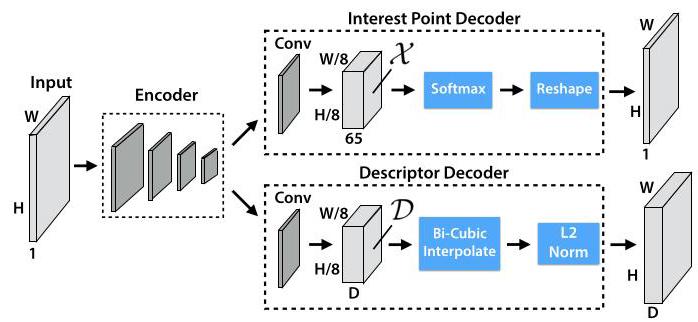
Figure 3. SuperPoint Decoders. Both decoders operate on a shared and spatially reduced representation of the input. To keep the model fast and easy to train, both decoders use non-learned upsampling to bring the representation back to \({\mathbb{R}}^{H \times W}\) .
图3. SuperPoint解码器。两个解码器都对输入的共享且空间维度降低的表示进行操作。为了使模型快速且易于训练,两个解码器都使用非学习的上采样将表示恢复到 \({\mathbb{R}}^{H \times W}\) 。
3.3. Descriptor Decoder
3.3. 描述符解码器
The descriptor head computes \(\mathcal{D} \in {\mathbb{R}}^{{H}_{c} \times {W}_{c} \times D}\) and outputs a tensor sized \({\mathbb{R}}^{H \times W \times D}\) . To output a dense map of L2- normalized fixed length descriptors, we use a model similar to UCN [3] to first output a semi-dense grid of descriptors (e.g., one every 8 pixels). Learning descriptors semi-densely rather than densely reduces training memory and keeps the run-time tractable. The decoder then performs bi-cubic interpolationof the descriptor and then L2-normalizes the activations to be unit length. This fixed, non-learned descriptor decoder is shown in Figure 3.
描述符头部计算 \(\mathcal{D} \in {\mathbb{R}}^{{H}_{c} \times {W}_{c} \times D}\) 并输出一个大小为 \({\mathbb{R}}^{H \times W \times D}\) 的张量。为了输出一个经过 L2 归一化的固定长度描述符的密集图,我们使用一个类似于 UCN [3] 的模型,首先输出一个半密集的描述符网格(例如,每 8 个像素一个)。以半密集而非密集的方式学习描述符可以减少训练内存,并使运行时间可控。然后,解码器对描述符进行双三次插值,然后将激活值进行 L2 归一化,使其长度为单位长度。这个固定的、不可学习的描述符解码器如图 3 所示。
3.4. Loss Functions
3.4. 损失函数
The final loss is the sum of two intermediate losses: one for the interest point detector, \({\mathcal{L}}_{p}\) , and one for the descriptor, \({\mathcal{L}}_{d}\) . We use pairs of synthetically warped images which have both (a) pseudo-ground truth interest point locations and (b) the ground truth correspondence from a randomly generated homography \(\mathcal{H}\) which relates the two images. This allows us to optimize the two losses simultaneously, given a pair of images, as shown in Figure 2c. We use \(\lambda\) to balance the final loss:
最终损失是两个中间损失的总和:一个是用于兴趣点检测器的 \({\mathcal{L}}_{p}\),另一个是用于描述符的 \({\mathcal{L}}_{d}\)。我们使用合成变形图像对,这些图像对同时具有 (a) 伪真实兴趣点位置和 (b) 由随机生成的单应性矩阵 \(\mathcal{H}\) 得到的真实对应关系,该单应性矩阵关联了这两幅图像。这使我们能够在给定一对图像的情况下同时优化这两个损失,如图 2c 所示。我们使用 \(\lambda\) 来平衡最终损失:
The interest point detector loss function \({\mathcal{L}}_{p}\) is a fully-convolutional cross-entropy loss over the cells \({\mathbf{x}}_{hw} \in \mathcal{X}\) . We call the set of corresponding ground-truth interest point labels \({}^{2}Y\) and individual entries as \({y}_{hw}\) . The loss is:
兴趣点检测器损失函数 \({\mathcal{L}}_{p}\) 是在单元格 \({\mathbf{x}}_{hw} \in \mathcal{X}\) 上的全卷积交叉熵损失。我们将对应的真实兴趣点标签集合称为 \({}^{2}Y\),将单个条目称为 \({y}_{hw}\)。损失为:
where
其中
\({}^{1}\) This decoder has no parameters, and is known as "sub-pixel convolution" [26] or "depth to space" in TensorFlow or "pixel shuffle" in PyTorch.
\({}^{1}\) 这个解码器没有参数,在 TensorFlow 中被称为“子像素卷积” [26] 或“深度到空间”,在 PyTorch 中被称为“像素洗牌”。
\({}^{2}\) If two ground truth corner positions land in the same bin then we randomly select one ground truth corner location.
\({}^{2}\) 如果两个真实角点位置落在同一个区间内,那么我们随机选择一个真实角点位置。
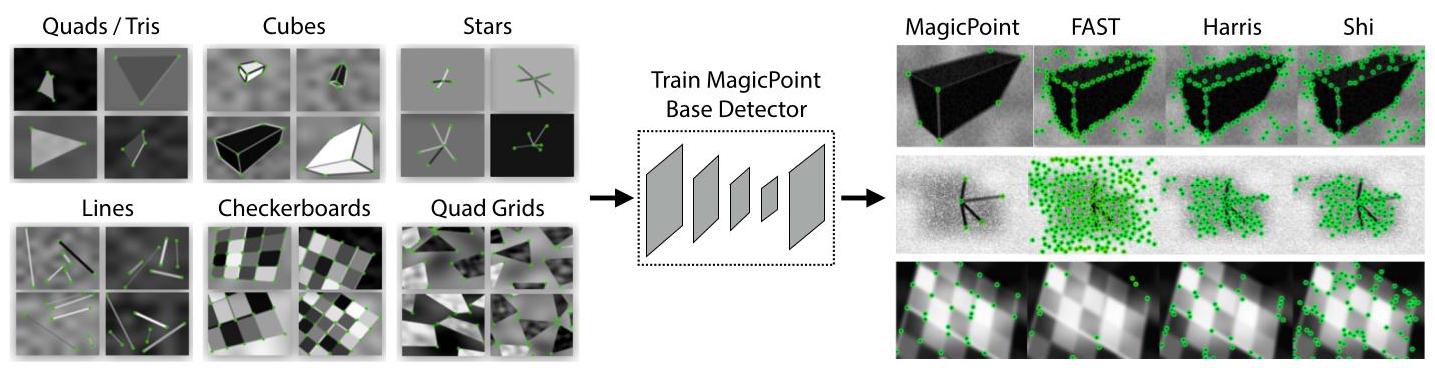
Figure 4. Synthetic Pre-Training. We use our Synthetic Shapes dataset consisting of rendered triangles, quadrilaterals, lines, cubes, checkerboards, and stars each with ground truth corner locations. The dataset is used to train the MagicPoint convolutional neural network, which is more robust to noise when compared to classical detectors.
图 4. 合成预训练。我们使用合成形状数据集,该数据集由渲染的三角形、四边形、直线、立方体、棋盘和星星组成,每个都有真实角点位置。该数据集用于训练 MagicPoint 卷积神经网络,与传统检测器相比,它对噪声更具鲁棒性。
The descriptor loss is applied to all pairs of descriptor cells, \({\mathbf{d}}_{hw} \in \mathcal{D}\) from the first image and \({\mathbf{d}}^{\prime }{}_{{h}^{\prime }{w}^{\prime }} \in {\mathcal{D}}^{\prime }\) from the second image. The homography-induced correspondence between the(h, w)cell and the \(\left( {{h}^{\prime },{w}^{\prime }}\right)\) cell can be written as follows:
描述符损失应用于所有描述符单元格对,第一幅图像中的 \({\mathbf{d}}_{hw} \in \mathcal{D}\) 和第二幅图像中的 \({\mathbf{d}}^{\prime }{}_{{h}^{\prime }{w}^{\prime }} \in {\mathcal{D}}^{\prime }\)。(h, w) 单元格和 \(\left( {{h}^{\prime },{w}^{\prime }}\right)\) 单元格之间由单应性引起的对应关系可以写成如下形式:
where \({\mathbf{p}}_{hw}\) denotes the location of the center pixel in the (h, w)cell, and \(\overset{⏜}{\mathcal{H}{\mathbf{p}}_{hw}}\) denotes multiplying the cell location \({\mathbf{p}}_{hw}\) by the homography \(\mathcal{H}\) and dividing by the last coordinate, as is usually done when transforming between Euclidean and homogeneous coordinates. We denote the entire set of correspondences for a pair of images with \(S\) .
其中 \({\mathbf{p}}_{hw}\) 表示 (h, w) 单元格中中心像素的位置,\(\overset{⏜}{\mathcal{H}{\mathbf{p}}_{hw}}\) 表示将单元格位置 \({\mathbf{p}}_{hw}\) 乘以单应性矩阵 \(\mathcal{H}\) 并除以最后一个坐标,这在欧几里得坐标和齐次坐标之间进行转换时通常会这样做。我们用 \(S\) 表示一对图像的整个对应关系集合。
We also add a weighting term \({\lambda }_{d}\) to help balance the fact that there are more negative correspondences than positive ones. We use a hinge loss with positive margin \({m}_{p}\) and negative margin \({m}_{n}\) . The descriptor loss is defined as:
我们还添加了一个加权项 \({\lambda }_{d}\) 来帮助平衡负对应关系比正对应关系更多的情况。我们使用具有正边界 \({m}_{p}\) 和负边界 \({m}_{n}\) 的铰链损失。描述符损失定义为:
where
其中
4. Synthetic Pre-Training
4. 合成预训练
In this section, we describe our method for training a base detector (shown in Figure 2a) called MagicPoint which is used in conjunction with Homographic Adaptation to generate pseudo-ground truth interest point labels for unlabeled images in a self-supervised fashion.
在本节中,我们描述了一种训练基础检测器(如图 2a 所示)的方法,该检测器称为 MagicPoint,它与单应性自适应结合使用,以自监督的方式为未标记图像生成伪真实兴趣点标签。
4.1. Synthetic Shapes
4.1. 合成形状
There is no large database of interest point labeled images that exists today. Thus to bootstrap our deep interest point detector, we first create a large-scale synthetic dataset called Synthetic Shapes that consists of simplified 2D geometry via synthetic data rendering of quadrilaterals, triangles, lines and ellipses. Examples of these shapes are shown in Figure 4. In this dataset, we are able to remove label ambiguity by modeling interest points with simple Y-junctions, L-junctions, T-junctions as well as centers of tiny ellipses and end points of line segments.
目前还没有大规模的兴趣点标注图像数据库。因此,为了启动我们的深度兴趣点检测器,我们首先创建了一个名为“合成形状(Synthetic Shapes)”的大规模合成数据集,该数据集通过对四边形、三角形、直线和椭圆进行合成数据渲染,由简化的二维几何图形组成。图4展示了这些形状的示例。在这个数据集中,我们能够通过用简单的Y形交点、L形交点、T形交点以及小椭圆的中心和线段的端点来建模兴趣点,从而消除标签的歧义性。
Once the synthetic images are rendered, we apply homographic warps to each image to augment the number of training examples. The data is generated on-the-fly and no example is seen by the network twice. While the types of interest points represented in Synthetic Shapes represents only a subset of all potential interest points found in the real world, we found it to work reasonably well in practice when used to train an interest point detector.
一旦合成图像渲染完成,我们对每个图像应用单应性变换(homographic warps)来增加训练样本的数量。数据是即时生成的,网络不会两次看到同一个样本。虽然“合成形状”数据集中表示的兴趣点类型仅代表现实世界中所有潜在兴趣点的一个子集,但我们发现在训练兴趣点检测器时,它在实践中表现相当不错。
4.2. MagicPoint
4.2. 魔法点(MagicPoint)
We use the detector pathway of the SuperPoint architecture (ignoring the descriptor head) and train it on Synthetic Shapes. We call the resulting model MagicPoint.
我们使用SuperPoint架构的检测器路径(忽略描述符头),并在“合成形状”数据集上对其进行训练。我们将得到的模型称为“魔法点(MagicPoint)”。
Interestingly, when we evaluate MagicPoint against other traditional corner detection approaches such as FAST [21], Harris corners [8] and Shi-Tomasi's "Good Features To Track" [25] on the Synthetic Shapes dataset, we discovered a large performance gap in our favor. We measure the mean Average Precision (mAP) on 1000 held-out images of the Synthetic Shapes dataset, and report the results in Table 2. The classical detectors struggle in the presence of imaging noise - qualitative examples of this are shown in Figure 4. More detailed experiments can be found in Appendix B.
有趣的是,当我们在“合成形状”数据集上,将“魔法点(MagicPoint)”与其他传统角点检测方法(如FAST [21]、哈里斯角点(Harris corners) [8] 和Shi - Tomasi的“适合跟踪的特征(Good Features To Track)” [25])进行评估比较时,我们发现“魔法点(MagicPoint)”具有明显的性能优势。我们在“合成形状”数据集的1000张保留图像上测量平均精度均值(mean Average Precision,mAP),并将结果列于表2中。经典检测器在存在成像噪声的情况下表现不佳——图4展示了这方面的定性示例。更详细的实验可在附录B中找到。
| MagicPoint | FAST | Harris | Shi | |
| mAPno noise | 0.979 | 0.405 | 0.678 | 0.686 |
| mAPnoise | 0.971 | 0.061 | 0.213 | 0.157 |
Table 2. Synthetic Shapes Detector Performance. The Magic-Point model outperforms classical detectors in detecting corners of simple geometric shapes and is robust to added noise.
表2. 合成形状检测器性能。“魔法点(Magic - Point)”模型在检测简单几何形状的角点方面优于经典检测器,并且对添加的噪声具有鲁棒性。
The MagicPoint detector performs very well on Synthetic Shapes, but does it generalize to real images? To summarize a result that we later present in Section 7.2, the answer is yes, but not as well as we hoped. We were surprised to find that MagicPoint performs reasonably well on real world images, especially on scenes which have strong corner-like structure such as tables, chairs and windows. Unfortunately in the space of all natural images, it under-performs when compared to the same classical detectors on repeatability under viewpoint changes. This motivated our self-supervised approach for training on real-world images which we call Homographic Adaptation.
“魔法点(MagicPoint)”检测器在“合成形状”数据集上表现非常好,但它能否推广到真实图像呢?总结我们将在7.2节中呈现的结果,答案是肯定的,但效果不如我们期望的那样好。我们惊讶地发现,“魔法点(MagicPoint)”在真实世界图像上表现相当不错,特别是在具有明显角状结构的场景中,如桌子、椅子和窗户。不幸的是,在所有自然图像的范围内,与相同的经典检测器相比,它在视角变化下的重复性方面表现较差。这促使我们采用一种自监督方法在真实世界图像上进行训练,我们称之为单应性自适应(Homographic Adaptation)。
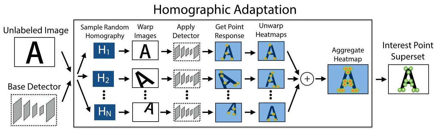
Figure 5. Homographic Adaptation. Homographic Adaptation is a form of self-supervision for boosting the geometric consistency of an interest point detector trained with convolutional neural networks. The entire procedure is mathematically defined in Equation 10.
图5. 单应性自适应(Homographic Adaptation)。单应性自适应是一种自监督形式,用于提高使用卷积神经网络训练的兴趣点检测器的几何一致性。整个过程在公式10中进行了数学定义。
5. Homographic Adaptation
5. 单应性自适应(Homographic Adaptation)
Our system bootstraps itself from a base interest point detector and a large set of unlabeled images from the target domain (e.g., MS-COCO). Operating in a self-supervised paradigm (also known as self-training), we first generate a set of pseudo-ground truth interest point locations for each image in the target domain, then use traditional supervised learning machinery. At the core of our method is a process that applies random homographies to warped copies of the input image and combines the results - a process we call Homographic Adaptation (see Figure 5).
我们的系统从一个基础兴趣点检测器和目标领域(例如,MS - COCO)的大量未标注图像中进行自启动。在自监督范式(也称为自训练)下运行,我们首先为目标领域中的每个图像生成一组伪真实兴趣点位置,然后使用传统的监督学习机制。我们方法的核心是一个过程,该过程对输入图像的变形副本应用随机单应性变换,并合并结果——我们将这个过程称为单应性自适应(见 图5)。
5.1. Formulation
5.1. 公式化表达
Homographies give exact or almost exact image-to-image transformations for camera motion with only rotation around the camera center, scenes with large distances to objects, and planar scenes. Moreover, because most of the world is reasonably planar, a homography is good model for what happens when the same 3D point is seen from different viewpoints. Because homographies do not require \(3\mathrm{D}\) information, they can be randomly sampled and easily applied to any 2D image - involving little more than bilinear interpolation. For these reasons, homographies are at the core of our self-supervised approach.
对于仅绕相机中心旋转的相机运动、与物体距离较远的场景以及平面场景,单应性变换(Homographies)能给出精确或近乎精确的图像到图像的变换。此外,由于现实世界的大部分区域近似为平面,当从不同视角观察同一个三维点时,单应性变换是一个很好的模型。因为单应性变换不需要 \(3\mathrm{D}\) 信息,所以可以对其进行随机采样并轻松应用于任何二维图像——只需要进行双线性插值。出于这些原因,单应性变换是我们自监督方法的核心。
Let \({f}_{\theta }\left( \cdot \right)\) represent the initial interest point function we wish to adapt, \(I\) the input image, \(\mathbf{x}\) the resulting interest points and \(\mathcal{H}\) a random homography, so that:
设 \({f}_{\theta }\left( \cdot \right)\) 表示我们希望进行自适应调整的初始兴趣点函数,\(I\) 表示输入图像,\(\mathbf{x}\) 表示得到的兴趣点,\(\mathcal{H}\) 表示一个随机单应性变换,那么:
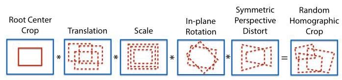
Figure 6. Random Homography Generation. We generate random homographies as the composition of less expressive, simple transformations.
图6. 随机单应性变换生成。我们将随机单应性变换生成为表达能力较弱的简单变换的组合。
An ideal interest point operator should be covariant with respect to homographies. A function \({f}_{\theta }\left( \cdot \right)\) is covariant with \(\mathcal{H}\) if the output transforms with the input. In other words, a covariant detector will satisfy, for all \({\mathcal{H}}^{3}\) :
一个理想的兴趣点算子应该相对于单应性变换具有协变性。如果一个函数 \({f}_{\theta }\left( \cdot \right)\) 的输出随输入进行变换,那么它相对于 \(\mathcal{H}\) 具有协变性。换句话说,一个具有协变性的检测器将满足,对于所有的 \({\mathcal{H}}^{3}\) :
moving homography-related terms to the right, we get:
将与单应性变换相关的项移到右边,我们得到:
In practice, a detector will not be perfectly covariant - different homographies in Equation 9 will result in different interest points \(\mathbf{x}\) . The basic idea behind Homographic Adaptation is to perform an empirical sum over a sufficiently large sample of random \(\mathcal{H}\) ’s (see Figure 5). The resulting aggregation over samples thus gives rise to a new and improved, super-point detector, \(\widehat{F}\left( \cdot \right)\) :
实际上,检测器不会具有完美的协变性——公式9中的不同单应性变换会导致不同的兴趣点 \(\mathbf{x}\) 。单应性自适应背后的基本思想是对足够大的随机 \(\mathcal{H}\) 样本进行经验求和(见图5)。因此,对样本进行的聚合产生了一种新的、改进后的超级点检测器 \(\widehat{F}\left( \cdot \right)\) :
5.2. Choosing Homographies
5.2. 选择单应性变换
Not all 3x3 matrices are good choices for Homographic Adaptation. To sample good homographies which represent plausible camera transformations, we decompose a potential homography into more simple, less expressive transformation classes. We sample within pre-determined ranges for translation, scale, in-plane rotation, and symmetric perspective distortion using a truncated normal distribution. These transformations are composed together with an initial root center crop to help avoid bordering artifacts. This process is shown in Figure 6.
并非所有3x3矩阵都适合用于单应性自适应。为了采样出能代表合理相机变换的良好单应性变换,我们将潜在的单应性变换分解为更简单、表达能力更弱的变换类别。我们使用截断正态分布在预先确定的平移、缩放、平面内旋转和对称透视畸变范围内进行采样。这些变换与初始的中心裁剪操作相结合,以避免出现边界伪影。这一过程如图6所示。
\({}^{3}\) For clarity, we slightly abuse notation and allow \(\mathcal{H}\mathbf{x}\) to denote the homography matrix \(\mathcal{H}\) being applied to the resulting interest points, and \(\mathcal{H}\left( I\right)\) to denote the entire image \(I\) being warped by \(\mathcal{H}\) .
\({}^{3}\) 为清晰起见,我们略微滥用一下符号,用 \(\mathcal{H}\mathbf{x}\) 表示应用于所得兴趣点的单应性矩阵 \(\mathcal{H}\) ,用 \(\mathcal{H}\left( I\right)\) 表示被 \(\mathcal{H}\) 进行单应性变换后的整个图像 \(I\) 。
When applying Homographic Adaptation to an image, we use the average response across a large number of homographic warps of the input image. The number of homographic warps \({N}_{h}\) is a hyper-parameter of our approach. We typically enforce the first homography to be equal to identity, so that \({N}_{h} = 1\) in our experiments corresponds to doing no adaptation. We performed an experiment to determine the best value for \({N}_{h}\) , varying the range of \({N}_{h}\) from small \({N}_{h} = {10}\) , to medium \({N}_{h} = {100}\) , and large \({N}_{h} = {1000}\) . Our experiments suggest that there is diminishing returns when performing more than 100 homographies. On a held-out set of images from MS-COCO, we obtain a repeatability score of .67 without any Homographic Adaptation, a repeatability boost of \({21}\%\) when performing \({N}_{h} = {100}\) transforms, and a repeatability boost of \({22}\%\) when \({N}_{h} = {1000}\) , thus the added benefit of using more than 100 homographies is minimal. For a more detailed analysis and discussion of this experiment see Appendix C.
将单应性自适应应用于图像时,我们使用输入图像经过大量单应性变换后的平均响应。单应性变换的数量 \({N}_{h}\) 是我们方法的一个超参数。我们通常强制第一个单应性变换为单位矩阵,这样在我们的实验中 \({N}_{h} = 1\) 就对应于不进行自适应。我们进行了一项实验来确定 \({N}_{h}\) 的最佳值,将 \({N}_{h}\) 的范围从较小的 \({N}_{h} = {10}\) 变化到中等的 \({N}_{h} = {100}\) ,再到较大的 \({N}_{h} = {1000}\) 。我们的实验表明,进行超过100次单应性变换时,收益会逐渐减少。在MS - COCO的一个保留图像集上,不进行任何单应性自适应时,我们的重复率得分是0.67;进行 \({N}_{h} = {100}\) 次变换时,重复率提升了 \({21}\%\) ;进行 \({N}_{h} = {1000}\) 次变换时,重复率提升了 \({22}\%\) ,因此使用超过100次单应性变换的额外收益很小。有关该实验的更详细分析和讨论,请参阅附录C。
5.3. Iterative Homographic Adaptation
5.3. 迭代单应性自适应
We apply the Homographic Adaptation technique at training time to improve the generalization ability of the base MagicPoint architecture on real images. The process can be repeated iteratively to continually self-supervise and improve the interest point detector. In all of our experiments, we call the resulting model, after applying Homographic Adaptation, SuperPoint and show the qualitative progression on images from HPatches in Figure 7.
我们在训练时应用单应性自适应技术,以提高基础MagicPoint架构在真实图像上的泛化能力。这个过程可以迭代进行,以持续进行自监督并改进兴趣点检测器。在我们所有的实验中,应用单应性自适应后得到的模型称为SuperPoint,图7展示了在HPatches图像上的定性进展。
6. Experimental Details
6. 实验细节
In this section we provide some implementation details for training the MagicPoint and SuperPoint models. This encoder has a VGG-like [27] architecture that has eight 3x3 convolution layers sized 64-64-64-64-128-128- 128-128. Every two layers there is a \(2 \times 2\) max pool layer. Each decoder head has a single \(3 \times 3\) convolutional layer of 256 units followed by a 1x1 convolution layer with 65 units and 256 units for the interest point detector and descriptor respectively. All convolution layers in the network are followed by ReLU non-linear activation and BatchNorm normalization.
在本节中,我们提供了训练MagicPoint和SuperPoint模型的一些实现细节。该编码器具有类似VGG [27] 的架构,包含八个3x3卷积层,尺寸为64 - 64 - 64 - 64 - 128 - 128 - 128 - 128。每两层之间有一个 \(2 \times 2\) 最大池化层。每个解码器头都有一个包含256个单元的 \(3 \times 3\) 卷积层,随后是一个1x1卷积层,兴趣点检测器和描述符的1x1卷积层分别有65个单元和256个单元。网络中的所有卷积层之后都跟着ReLU非线性激活函数和批量归一化(BatchNorm)操作。
To train the fully-convolutional SuperPoint model, we start with a base MagicPoint model trained on Synthetic Shapes. The MagicPoint architecture is the SuperPoint architecture without the descriptor head. The MagicPoint model is trained for 200,000 iterations of synthetic data. Since the synthetic data is simple and fast to render, the data is rendered on-the-fly, thus no single example is seen twice by the network.
为了训练全卷积的SuperPoint模型,我们从在合成形状上训练的基础MagicPoint模型开始。MagicPoint架构是没有描述符头的SuperPoint架构。MagicPoint模型在合成数据上训练200,000次迭代。由于合成数据简单且渲染速度快,数据是实时渲染的,因此网络不会两次看到同一个样本。
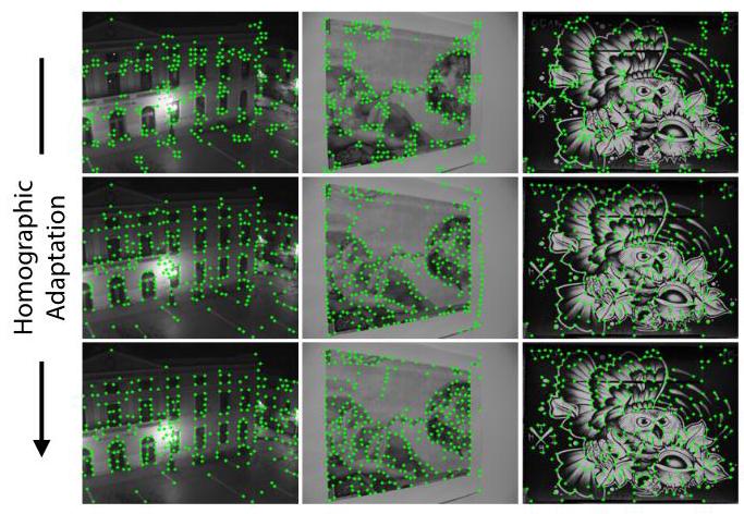
Figure 7. Iterative Homographic Adaptation. Top row: initial base detector (MagicPoint) struggles to find repeatable detections. Middle and bottom rows: further training with Homographic Adaption improves detector performance.
图7. 迭代单应性自适应。第一行:初始的基础检测器(MagicPoint)难以找到可重复的检测结果。中间行和底行:通过单应性自适应进行进一步训练可提高检测器性能。
We generate pseudo-ground truth labels using the MS-COCO 2014 [13] training dataset split which has 80,000 images and the MagicPoint base detector. The images are sized to a resolution of \({240} \times {320}\) and converted to grayscale. The labels are generated using Homographic Adaptation with \({N}_{h} = {100}\) , as motivated by our results from Section 5.2. We repeat the Homographic Adaptation a second time, using the resulting model trained from the first round of Homographic Adaptation.
我们使用MS - COCO 2014 [13]训练数据集划分(包含80,000张图像)和MagicPoint基础检测器生成伪真实标签。将图像调整为\({240} \times {320}\)分辨率并转换为灰度图。受5.2节结果的启发,使用具有\({N}_{h} = {100}\)的单应性自适应方法生成标签。我们使用第一轮单应性自适应训练得到的模型,再次进行单应性自适应。
The joint training of SuperPoint is also done on \({240} \times {320}\) grayscale COCO images. For each training example, a homography is randomly sampled. It is sampled from a more restrictive set of homographies than during Homographic Adaptation to better model the target application of pairwise matching (e.g., we avoid sampling extreme in-plane rotations as they are rarely seen in HPatches). The image and corresponding pseudo-ground truth are transformed by the homography to create the needed inputs and labels. The descriptor size used in all experiments is \(D = {256}\) . We use a weighting term of \({\lambda }_{d} = {250}\) to keep the descriptor learning balanced. The descriptor hinge loss uses a positive margin \({m}_{p} = 1\) and negative margin \({m}_{n} = {0.2}\) . We use a factor of \(\lambda = {0.0001}\) to balance the two losses.
SuperPoint的联合训练同样在\({240} \times {320}\)灰度COCO图像上进行。对于每个训练样本,随机采样一个单应性矩阵。与单应性自适应过程相比,这里从更严格的单应性矩阵集合中采样,以便更好地模拟成对匹配的目标应用(例如,我们避免采样极端的平面内旋转,因为在HPatches中很少出现这种情况)。通过单应性变换对图像和相应的伪真实标签进行转换,以创建所需的输入和标签。所有实验中使用的描述符大小为\(D = {256}\)。我们使用\({\lambda }_{d} = {250}\)的加权项来保持描述符学习的平衡。描述符的铰链损失使用正边界\({m}_{p} = 1\)和负边界\({m}_{n} = {0.2}\)。我们使用\(\lambda = {0.0001}\)的因子来平衡这两种损失。
All training is done using PyTorch [19] with mini-batch sizes of 32 and the ADAM solver with default parameters of \({lr} = {0.001}\) and \(\beta = \left( {{0.9},{0.999}}\right)\) . We also use standard data augmentation techniques such as random Gaussian noise, motion blur, brightness level changes to improve the network's robustness to lighting and viewpoint changes.
所有训练均使用PyTorch [19]进行,小批量大小为32,使用ADAM求解器,默认参数为\({lr} = {0.001}\)和\(\beta = \left( {{0.9},{0.999}}\right)\)。我们还使用标准的数据增强技术,如随机高斯噪声、运动模糊、亮度级别变化,以提高网络对光照和视角变化的鲁棒性。
| 57 Illumination Scenes | 59 Viewpoint Scenes | |||
| NMS=4 | NMS=8 | NMS=4 | NMS=8 | |
| SuperPoint | .652 | .631 | .503 | .484 |
| MagicPoint | .575 | .507 | .322 | .260 |
| ${FAST}$ | .575 | .472 | .503 | .404 |
| Harris | .620 | .533 | .556 | .461 |
| Shi | .606 | .511 | .552 | .453 |
| Random | .101 | .103 | .100 | .104 |
Table 3. HPatches Detector Repeatability. SuperPoint is the most repeatable under illumination changes, competitive on viewpoint changes, and outperforms MagicPoint in all scenarios.
表3. HPatches检测器的可重复性。SuperPoint在光照变化下的可重复性最高,在视角变化下具有竞争力,并且在所有场景中都优于MagicPoint。
7. Experiments
7. 实验
In this section we present quantitative results of the methods presented in the paper. Evaluation of interest points and descriptors is a well-studied topic, thus we follow the evaluation protocol of Mikolajczyk et al. [16]. For more details on our evaluation metrics, see Appendix A.
在本节中,我们展示了本文所提出方法的定量结果。兴趣点和描述符的评估是一个经过深入研究的主题,因此我们遵循Mikolajczyk等人[16]的评估协议。有关我们评估指标的更多详细信息,请参阅附录A。
7.1. System Runtime
7.1. 系统运行时间
We measure the run-time of the SuperPoint architecture using a Titan X GPU and the timing tool that comes with the Caffe [11] deep learning library. A single forward pass of the model runs in approximately \({11.15}\mathrm{\;{ms}}\) with inputs sized \({480} \times {640}\) , which produces the point detection locations and a semi-dense descriptor map. To sample the descriptors at the higher \({480} \times {640}\) resolution from the semi-dense descriptor, it is not necessary to create the entire dense descriptor map - we can just sample from the 1000 detected locations, which takes about \({1.5}\mathrm{\;{ms}}\) on a CPU implementation of bi-cubic interpolation followed by L2 normalization. Thus we estimate the total runtime of the system on a GPU to be about \({13}\mathrm{\;{ms}}\) or \({70}\mathrm{{FPS}}\) .
我们使用Titan X GPU和Caffe [11]深度学习库附带的计时工具来测量SuperPoint架构的运行时间。模型的单次前向传播在输入大小为\({480} \times {640}\)的情况下大约需要\({11.15}\mathrm{\;{ms}}\),这会产生点检测位置和半密集描述符图。为了从半密集描述符中以更高的\({480} \times {640}\)分辨率采样描述符,无需创建整个密集描述符图 - 我们只需从1000个检测位置进行采样,在CPU上进行双三次插值并进行L2归一化大约需要\({1.5}\mathrm{\;{ms}}\)。因此,我们估计系统在GPU上的总运行时间约为\({13}\mathrm{\;{ms}}\)或\({70}\mathrm{{FPS}}\)。
7.2. HPatches Repeatability
7.2. HPatches可重复性
In our experiments we train SuperPoint on the MS-COCO images, and evaluate using the HPatches dataset [2]. HPatches contains 116 scenes with 696 unique images. The first 57 scenes exhibit large changes in illumination and the other 59 scenes have large viewpoint changes.
在我们的实验中,我们在MS - COCO图像上训练SuperPoint,并使用HPatches数据集[2]进行评估。HPatches包含116个场景,共696张独特的图像。前57个场景表现出较大的光照变化,另外59个场景有较大的视角变化。
To evaluate the interest point detection ability of the Su-perPoint model, we measure repeatability on the HPatches dataset. We compare it to the MagicPoint model (before Homographic Adaptation), as well as FAST [21], Harris [8] and Shi [25], all implemented using OpenCV. Repeatability is computed at \({240} \times {320}\) resolution with 300 points detected in each image. We also vary the Non-Maximum Suppression (NMS) applied to the detections. We use a correct distance of \(\epsilon = 3\) pixels. Applying larger amounts of NMS helps ensure that the points are evenly distributed in the image, useful for certain applications such as ORB-SLAM [17], where a minimum number of FAST corner detections is forced in each cell of a coarse grid.
为了评估SuperPoint模型的兴趣点检测能力,我们在HPatches数据集上测量可重复性。我们将其与MagicPoint模型(单应性自适应之前)以及使用OpenCV实现的FAST [21]、Harris [8]和Shi [25]进行比较。可重复性在\({240} \times {320}\)分辨率下计算,每张图像检测300个点。我们还改变了应用于检测结果的非极大值抑制(NMS)。我们使用\(\epsilon = 3\)像素的正确距离。应用更多的NMS有助于确保点在图像中均匀分布,这对于某些应用(如ORB - SLAM [17])很有用,在这些应用中,会在粗网格的每个单元格中强制检测最少数量的FAST角点。
| Homography Estimation | Detector Metrics | Descriptor Metrics | |||||
| $\epsilon = 1$ | $\epsilon = 3$ | $\epsilon = 5$ | Rep. | MLE | NN mAP | M. Score | |
| SuperPoint | .310 | .684 | .829 | .581 | 1.158 | .821 | .470 |
| LIFT | .284 | .598 | .717 | .449 | 1.102 | .664 | .315 |
| SIFT | .424 | .676 | .759 | .495 | 0.833 | .694 | .313 |
| ${ORB}$ | .150 | .395 | .538 | .641 | 1.157 | .735 | .266 |
Table 4. HPatches Homography Estimation. SuperPoint outperforms LIFT and ORB and performs comparably to SIFT using various \(\epsilon\) thresholds of correctness. We also report related metrics which measure detector and descriptor performance individually.
表4. HPatches单应性估计。在使用各种\(\epsilon\)正确阈值的情况下,SuperPoint的性能优于LIFT和ORB,并且与SIFT相当。我们还报告了分别衡量检测器和描述符性能的相关指标。
In summary, the Homographic Adaptation technique used to transform MagicPoint into SuperPoint gives a large boost in repeatability, especially under large viewpoint changes. Results are shown in Table 3. The SuperPoint model outperforms classical detectors under illumination changes and performs on par with classical detectors under viewpoint changes.
总之,用于将MagicPoint转换为SuperPoint的单应性自适应技术显著提高了可重复性,尤其是在大视角变化的情况下。结果如表3所示。SuperPoint模型在光照变化的情况下性能优于传统检测器,在视角变化的情况下与传统检测器表现相当。
7.3. HPatches Homography Estimation
7.3. HPatches单应性估计
To evaluate the performance of the SuperPoint interest point detector and descriptor network, we compare matching ability on the HPatches dataset. We evaluate Su-perPoint against three well-known detector and descriptor systems: LIFT [32], SIFT [15] and ORB [22]. For LIFT we use the pre-trained model (Picadilly) provided by the authors. For SIFT and ORB we use the default OpenCV implementations. We use a correct distance of \(\epsilon = 3\) pixels for Rep, MLE, NN mAP and MScore. We compute a maximum of 1000 points for all systems at a \({480} \times {640}\) resolution and compute a number of metrics for each image pair. To estimate the homography, we perform nearest neighbor matching from all interest points+descriptors detected in the first image to all the interest points+descriptors in the second. We use an OpenCV implementation (findHomography ( ) with RANSAC) with all the matches to compute the final homography estimate.
为了评估SuperPoint兴趣点检测器和描述符网络的性能,我们在HPatches数据集上比较了匹配能力。我们将SuperPoint与三种著名的检测器和描述符系统进行了比较:LIFT [32]、SIFT [15]和ORB [22]。对于LIFT,我们使用作者提供的预训练模型(皮卡迪利模型)。对于SIFT和ORB,我们使用OpenCV的默认实现。对于重复率(Rep)、最大似然估计(MLE)、最近邻平均精度均值(NN mAP)和匹配得分(MScore),我们使用\(\epsilon = 3\)像素的正确距离。我们在\({480} \times {640}\)分辨率下为所有系统计算最多1000个点,并为每对图像计算多个指标。为了估计单应性,我们将第一张图像中检测到的所有兴趣点+描述符与第二张图像中的所有兴趣点+描述符进行最近邻匹配。我们使用OpenCV的实现(带有随机抽样一致性(RANSAC)的findHomography()函数),结合所有匹配来计算最终的单应性估计。
The homography estimation results are shown in Table 4. SuperPoint outperforms LIFT and ORB and performs comparably to SIFT for homography estimation on HPatches using various \(\epsilon\) thresholds of correctness. Qualitative examples of SuperPoint versus LIFT, SIFT and ORB are shown in Figure 8. Please see Appendix D for even more homography estimation example pairs. SuperPoint tends to produce a larger number of correct matches which densely cover the image, and is especially effective against illumination changes.
单应性估计结果如表4所示。在HPatches数据集上进行单应性估计时,使用各种\(\epsilon\)正确阈值,SuperPoint的性能优于LIFT和ORB,并且与SIFT相当。图8展示了SuperPoint与LIFT、SIFT和ORB的定性对比示例。更多单应性估计示例对请参见附录D。SuperPoint倾向于产生大量正确匹配,这些匹配密集地覆盖图像,并且在应对光照变化方面特别有效。
Quantitatively we outperform LIFT in almost all metrics. LIFT is also outperformed by SIFT in most metrics. This may be due to the fact that HPatches includes indoor sequences and LIFT was trained on a single outdoor sequence. Our method was trained on hundreds of thousands of warped MS-COCO images that exhibit a much larger diversity and more closely match the diversity in HPatches.
从数量上看,我们的方法在几乎所有指标上都优于LIFT。在大多数指标上,LIFT也不如SIFT。这可能是因为HPatches包含室内序列,而LIFT是在单个室外序列上训练的。我们的方法是在数十万张经过变换的MS - COCO图像上训练的,这些图像具有更大的多样性,并且与HPatches中的多样性更接近。
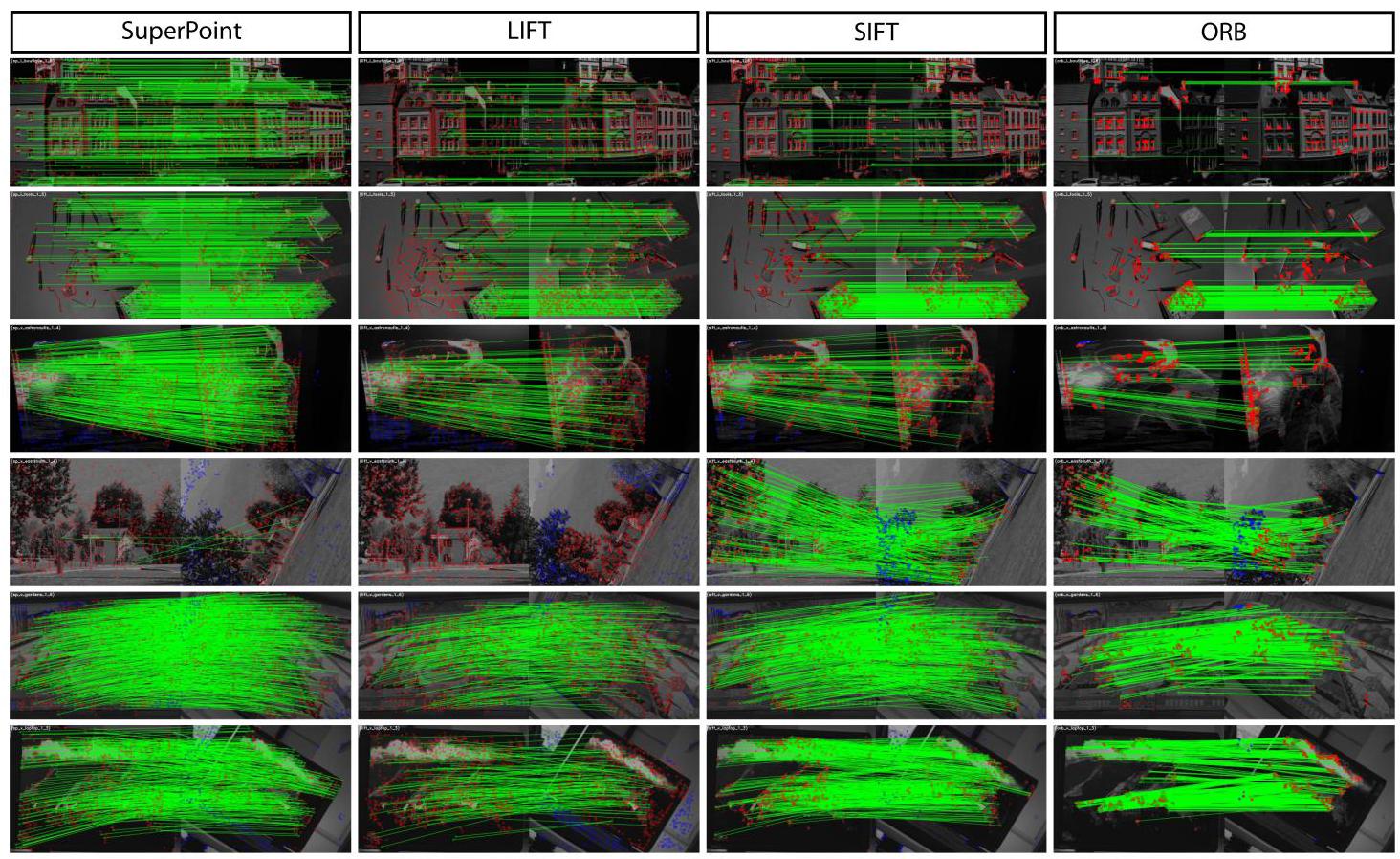
Figure 8. Qualitative Results on HPatches. The green lines show correct correspondences. SuperPoint tends to produce more dense and correct matches compared to LIFT, SIFT and ORB. While ORB has the highest average repeatability, the detections cluster together and generally do not result in more matches or more accurate homography estimates (see 4). Row 4: Failure case of SuperPoint and LIFT due to extreme in-plane rotation not seen in the training examples. See Appendix D for additional homography estimation example pairs.
图8. HPatches上的定性结果。绿色线条表示正确的对应关系。与LIFT、SIFT和ORB相比,SuperPoint倾向于产生更密集且正确的匹配。虽然ORB具有最高的平均可重复性,但检测结果会聚集在一起,通常不会产生更多的匹配或更准确的单应性估计(见4)。第4行:由于训练示例中未出现的极端平面内旋转,SuperPoint和LIFT出现失败情况。有关额外的单应性估计示例对,请参阅附录D。
SIFT performs well for sub-pixel precision homogra-phies \(\epsilon = 1\) and has the lowest mean localization error (MLE). This is likely due to the fact that SIFT performs extra sub-pixel localization, while other methods do not perform this step.
SIFT在亚像素精度单应性 \(\epsilon = 1\) 方面表现良好,并且具有最低的平均定位误差(MLE)。这可能是因为SIFT执行了额外的亚像素定位,而其他方法没有执行这一步骤。
ORB achieves the highest repeatability (Rep.); however, its detections tend to form sparse clusters throughout the image as shown in Figure 8, thus scoring poorly on the final homography estimation task. This suggests that optimizing solely for repeatability does not result in better matching or estimation further up the pipeline.
ORB实现了最高的可重复性(Rep.);然而,如图8所示,其检测结果倾向于在整个图像中形成稀疏的聚类,因此在最终的单应性估计任务中得分较低。这表明仅针对可重复性进行优化并不能在后续流程中带来更好的匹配或估计效果。
SuperPoint scores strongly in descriptor-focused metrics such as nearest neighbor mAP (NN mAP) and matching score (M. Score), which confirms findings from both Choy et al. [3] and Yi et al. [32] which show that learned representations for descriptor matching outperform hand-tuned representations.
SuperPoint在以描述符为重点的指标上得分很高,如最近邻平均精度均值(NN mAP)和匹配得分(M. Score),这证实了Choy等人[3]和Yi等人[32]的研究结果,即用于描述符匹配的学习表示优于手工调整的表示。
8. Conclusion
8. 结论
We have presented a fully-convolutional neural network architecture for interest point detection and description trained using a self-supervised domain adaptation framework called Homographic Adaptation. Our experiments demonstrate that (1) it is possible to transfer knowledge from a synthetic dataset onto real-world images, (2) sparse interest point detection and description can be cast as a single, efficient convolutional neural network, and (3) the resulting system works well for geometric computer vision matching tasks such as Homography Estimation.
我们提出了一种全卷积神经网络架构,用于兴趣点检测和描述,该架构使用一种名为单应性自适应(Homographic Adaptation)的自监督域自适应框架进行训练。我们的实验表明:(1)可以将知识从合成数据集迁移到真实世界的图像上;(2)稀疏兴趣点检测和描述可以作为一个高效的卷积神经网络来实现;(3)由此产生的系统在诸如单应性估计等几何计算机视觉匹配任务中表现良好。
Future work will investigate whether Homographic Adaptation can boost the performance of models such as those used in semantic segmentation (e.g., SegNet [1] ) and object detection (e.g., SSD [14]). It will also carefully investigate the ways that interest point detection and description (and potentially other tasks) benefit each other.
未来的工作将研究单应性自适应是否可以提升语义分割(如SegNet [1])和目标检测(如SSD [14])等模型的性能。还将仔细研究兴趣点检测和描述(以及潜在的其他任务)如何相互受益。
Lastly, we believe that our SuperPoint network can be used to tackle all visual data-association in 3D computer vision problems like SLAM and SfM, and that a learning-based Visual SLAM front-end will enable more robust applications in robotics and augmented reality.
最后,我们相信我们的SuperPoint网络可用于解决3D计算机视觉问题(如SLAM和SfM)中的所有视觉数据关联问题,并且基于学习的视觉SLAM前端将使机器人和增强现实领域的应用更加稳健。
References
参考文献
[1] V. Badrinarayanan, A. Kendall, and R. Cipolla. Seg-Net: A deep convolutional encoder-decoder architecture for image segmentation. PAMI, 2017. 3, 8
[1] V. Badrinarayanan、A. Kendall和R. Cipolla。Seg-Net:一种用于图像分割的深度卷积编解码器架构。《模式分析与机器智能汇刊》(PAMI),2017年。第3、8页
[2] V. Balntas, K. Lenc, A. Vedaldi, and K. Mikola-jczyk. HPatches: A benchmark and evaluation of handcrafted and learned local descriptors. In CVPR, 2017. 7
[2] V. Balntas、K. Lenc、A. Vedaldi和K. Mikolajczyk。HPatches:对手工和学习的局部描述符的基准测试和评估。发表于《计算机视觉与模式识别会议》(CVPR),2017年。第7页
[3] C. B. Choy, J. Gwak, S. Savarese, and M. Chandraker. Universal Correspondence Network. In NIPS. 2016. 2,3,8
[3] C. B. Choy、J. Gwak、S. Savarese和M. Chandraker。通用对应网络。发表于《神经信息处理系统大会》(NIPS),2016年。第2、3、8页
[4] D. DeTone, T. Malisiewicz, and A. Rabinovich. Deep image homography estimation. arXiv preprint arXiv:1606.03798, 2016. 2
[4] D. DeTone、T. Malisiewicz和A. Rabinovich。深度图像单应性估计。预印本arXiv:1606.03798,2016年。第2页
[5] D. DeTone, T. Malisiewicz, and A. Rabinovich. Toward geometric deepslam. arXiv preprint arXiv:1707.07410, 2017. 10
[5] D. DeTone、T. Malisiewicz和A. Rabinovich。迈向几何深度SLAM。预印本arXiv:1707.07410,2017年。第10页
[6] L. F. I. K. P. F. F. M.-N. Edgar Simo-Serra, Eduard Trulls. Discriminative learning of deep convolutional feature point descriptors. In \({ICCV},{2015.2}\)
[6] L. F. I. K. P. F. F. M.-N. Edgar Simo-Serra、Eduard Trulls。深度卷积特征点描述符的判别式学习。发表于 \({ICCV},{2015.2}\)
[7] Y. Ganin and V. Lempitsky. Unsupervised domain adaptation by backpropagation. In \({ICML},{2015.2}\)
[7] Y. Ganin和V. Lempitsky。通过反向传播进行无监督域自适应。发表于 \({ICML},{2015.2}\)
[8] C. Harris and M. Stephens. A combined corner and edge detector. In Alvey vision conference, volume 15, pages 10-5244. Manchester, UK, 1988. 4, 7, 10
[8] C. 哈里斯(C. Harris)和 M. 斯蒂芬斯(M. Stephens)。一种角点与边缘联合检测器。载于《阿尔维视觉会议论文集》(Alvey vision conference),第 15 卷,第 10 - 5244 页。英国曼彻斯特,1988 年。4, 7, 10
[9] R. Hartley and A. Zisserman. Multiple View Geometry in computer vision. 2003. 1
[9] R. 哈特利(R. Hartley)和 A. 齐瑟曼(A. Zisserman)。《计算机视觉中的多视图几何》(Multiple View Geometry in computer vision)。2003 年。1
[10] S. Honari, P. Molchanov, S. Tyree, P. Vincent, C. Pal, and J. Kautz. Improving landmark localization with semi-supervised learning. arXiv preprint arXiv:1709.01591, 2017. 2
[10] S. 霍纳里(S. Honari)、P. 莫尔恰诺夫(P. Molchanov)、S. 泰里(S. Tyree)、P. 文森特(P. Vincent)、C. 帕尔(C. Pal)和 J. 考茨(J. Kautz)。利用半监督学习改进地标定位。预印本 arXiv:1709.01591,2017 年。2
[11] Y. Jia, E. Shelhamer, J. Donahue, S. Karayev, J. Long, R. Girshick, S. Guadarrama, and T. Darrell. Caffe: Convolutional architecture for fast feature embedding. arXiv preprint arXiv:1408.5093, 2014. 7
[11] Y. 贾(Y. Jia)、E. 谢尔哈默(E. Shelhamer)、J. 多纳休(J. Donahue)、S. 卡拉耶夫(S. Karayev)、J. 朗(J. Long)、R. 吉里什克(R. Girshick)、S. 瓜达拉马(S. Guadarrama)和 T. 达雷尔(T. Darrell)。Caffe:用于快速特征嵌入的卷积架构。预印本 arXiv:1408.5093,2014 年。7
[12] C.-Y. Lee, V. Badrinarayanan, T. Malisiewicz, and A. Rabinovich. RoomNet: End-to-end room layout estimation. In \({ICCV},{2017.1}\)
[12] C.-Y. 李(C.-Y. Lee)、V. 巴德里纳拉亚南(V. Badrinarayanan)、T. 马利塞维奇(T. Malisiewicz)和 A. 拉宾诺维奇(A. Rabinovich)。RoomNet:端到端房间布局估计。载于 \({ICCV},{2017.1}\)
[13] T.-Y. Lin, M. Maire, S. Belongie, J. Hays, P. Perona, D. Ramanan, P. Dollár, and L. Zitnick. Microsoft COCO: Common objects in context. In \({ECCV},{2014}\) . 6
[13] T.-Y. 林(T.-Y. Lin)、M. 梅尔(M. Maire)、S. 贝隆吉(S. Belongie)、J. 海斯(J. Hays)、P. 佩罗纳(P. Perona)、D. 拉马南(D. Ramanan)、P. 多尔(P. Dollár)和 L. 齐特尼克(L. Zitnick)。微软 COCO:上下文中的常见物体。载于 \({ECCV},{2014}\) 。6
[14] W. Liu, D. Anguelov, D. Erhan, C. Szegedy, S. Reed, C.-Y. Fu, and A. C. Berg. SSD: Single shot multibox detector. In \({ECCV},{2016.1},8\)
[14] W. 刘(W. Liu)、D. 安格洛夫(D. Anguelov)、D. 埃尔汗(D. Erhan)、C. 塞格迪(C. Szegedy)、S. 里德(S. Reed)、C.-Y. 傅(C.-Y. Fu)和 A. C. 伯格(A. C. Berg)。SSD:单阶段多框检测器。载于 \({ECCV},{2016.1},8\)
[15] D. G. Lowe. Distinctive image features from scale-invariant keypoints. IJCV, 2004. 2, 7
[15] D. G. 洛(D. G. Lowe)。基于尺度不变关键点的独特图像特征。《国际计算机视觉杂志》(IJCV),2004 年。2, 7
[16] K. Mikolajczyk and C. Schmid. A performance evaluation of local descriptors. PAMI, 2005. 2, 7, 10
[16] K. 米科拉伊奇克(K. Mikolajczyk)和 C. 施密德(C. Schmid)。局部描述符的性能评估。《模式分析与机器智能汇刊》(PAMI),2005 年。2, 7, 10
[17] R. Mur-Artal, J. Montiel, and J. D. Tardos. ORB-SLAM: a versatile and accurate monocular SLAM system. IEEE Transactions on Robotics, 2015. 7
[17] R. 穆尔 - 阿塔尔(R. Mur-Artal)、J. 蒙蒂埃尔(J. Montiel)和 J. D. 塔尔多斯(J. D. Tardos)。ORB - SLAM:一种通用且准确的单目 SLAM 系统。《IEEE 机器人学汇刊》(IEEE Transactions on Robotics),2015 年。7
[18] A. Odena, V. Dumoulin, and C. Olah. Deconvolution and checkerboard artifacts. Distill, 2016. 3
[18] A. 奥德纳(A. Odena)、V. 杜穆林(V. Dumoulin)和 C. 奥拉(C. Olah)。反卷积与棋盘格伪影。《Distill》,2016 年。3
[19] A. Paszke, S. Gross, S. Chintala, and G. Chanan. PyTorch. https://github.com/pytorch/ pytorch. 6
[19] A. 帕斯齐克(A. Paszke)、S. 格罗斯(S. Gross)、S. 钦塔拉(S. Chintala)和 G. 查南(G. Chanan)。PyTorch。https://github.com/pytorch/ pytorch。6
[20] I. Rocco, R. Arandjelović, and J. Sivic. Convolutional neural network architecture for geometric matching. In \({CVPR},{2017.2}\)
[20] I. 罗科(I. Rocco)、R. 阿兰德耶洛维奇(R. Arandjelović)和 J. 西维奇(J. Sivic)。用于几何匹配的卷积神经网络架构。载于 \({CVPR},{2017.2}\)
[21] E. Rosten and T. Drummond. Machine learning for high-speed corner detection. In \({ECCV},{2006.2},4,7\) , 10
[21] E. 罗斯滕(E. Rosten)和 T. 德拉蒙德(T. Drummond)。用于高速角点检测的机器学习。载于 \({ECCV},{2006.2},4,7\) ,10
[22] E. Rublee, V. Rabaud, K. Konolige, and G. Bradski. ORB: An efficient alternative to SIFT or SURF. In ICCV, 2011. 7
[22] E. 鲁布利(E. Rublee)、V. 拉博(V. Rabaud)、K. 科诺利奇(K. Konolige)和 G. 布拉德斯基(G. Bradski)。ORB:SIFT 或 SURF 的高效替代方案。载于《国际计算机视觉会议论文集》(ICCV),2011 年。7
[23] N. Savinov, A. Seki, L. Ladicky, T. Sattler, and M. Pollefeys. Quad-networks: unsupervised learning to rank for interest point detection. In CVPR. 2017. 2
[23] N. 萨维诺夫(N. Savinov)、A. 关(A. Seki)、L. 拉迪基(L. Ladicky)、T. 萨特勒(T. Sattler)和 M. 波勒菲斯(M. Pollefeys)。Quad - 网络:用于兴趣点检测的无监督排序学习。载于《计算机视觉与模式识别会议论文集》(CVPR)。2017 年。2
[24] C. Schmid, R. Mohr, and C. Bauckhage. Evaluation of interest point detectors. IJCV, 2000. 2
[24] C. 施密德(C. Schmid)、R. 莫尔(R. Mohr)和 C. 鲍克哈格(C. Bauckhage)。兴趣点检测器的评估。《国际计算机视觉杂志》(IJCV),2000 年。2
[25] J. Shi and C. Tomasi. Good features to track. In CVPR, 1994. 4, 7, 10
[25] J. 石(J. Shi)和 C. 托马西(C. Tomasi)。适合跟踪的特征。见《计算机视觉与模式识别会议》(CVPR),1994 年。4, 7, 10
[26] W. Shi, J. Caballero, F. Huszár, J. Totz, A. P. Aitken, R. Bishop, D. Rueckert, and Z. Wang. Real-time single image and video super-resolution using an efficient sub-pixel convolutional neural network. In CVPR, 2016. 3
[26] W. 石(W. Shi)、J. 卡瓦列罗(J. Caballero)、F. 胡萨尔(F. Huszár)、J. 托茨(J. Totz)、A. P. 艾特肯(A. P. Aitken)、R. 毕晓普(R. Bishop)、D. 吕克特(D. Rueckert)和 Z. 王(Z. Wang)。使用高效亚像素卷积神经网络的实时单图像和视频超分辨率。见《计算机视觉与模式识别会议》(CVPR),2016 年。3
[27] K. Simonyan and A. Zisserman. Very deep convolutional networks for large-scale image recognition. arXiv preprint arXiv:1409.1556, 2014. 3, 6
[27] K. 西蒙扬(K. Simonyan)和 A. 齐斯曼(A. Zisserman)。用于大规模图像识别的非常深的卷积网络。预印本 arXiv:1409.1556,2014 年。3, 6
[28] B. Ummenhofer, H. Zhou, J. Uhrig, N. Mayer, E. Ilg, A. Dosovitskiy, and T. Brox. DeMoN: Depth and motion network for learning monocular stereo. In CVPR, 2017. 2
[28] B. 乌门霍费尔(B. Ummenhofer)、H. 周(H. Zhou)、J. 乌里希(J. Uhrig)、N. 迈尔(N. Mayer)、E. 伊尔格(E. Ilg)、A. 多索维茨基(A. Dosovitskiy)和 T. 布罗克斯(T. Brox)。DeMoN:用于学习单目立体视觉的深度和运动网络。见《计算机视觉与模式识别会议》(CVPR),2017 年。2
[29] Y. Verdie, K. Yi, P. Fua, and V. Lepetit. TILDE: A Temporally Invariant Learned DEtector. In CVPR, 2015.2
[29] Y. 韦尔迪(Y. Verdie)、K. 易(K. Yi)、P. 富阿(P. Fua)和 V. 勒佩蒂(V. Lepetit)。TILDE:一种时间不变的学习型检测器。见《计算机视觉与模式识别会议》(CVPR),2015 年。2
[30] S. Vijayanarasimhan, S. Ricco, C. Schmid, R. Suk-thankar, and K. Fragkiadaki. SfM-Net: Learning of structure and motion from video. arXiv preprint arXiv:1704.07804, 2017. 2
[30] S. 维贾亚纳拉西姆汉(S. Vijayanarasimhan)、S. 里科(S. Ricco)、C. 施密德(C. Schmid)、R. 苏克坦卡尔(R. Suk-thankar)和 K. 弗拉基阿达基(K. Fragkiadaki)。SfM-Net:从视频中学习结构和运动。预印本 arXiv:1704.07804,2017 年。2
[31] S.-E. Wei, V. Ramakrishna, T. Kanade, and Y. Sheikh. Convolutional pose machines. In \({CVPR},{2016.1}\)
[31] S.-E. 魏(S.-E. Wei)、V. 拉马克里希纳(V. Ramakrishna)、T. 卡纳德(T. Kanade)和 Y. 谢赫(Y. Sheikh)。卷积姿态机。见 \({CVPR},{2016.1}\)
[32] K. M. Yi, E. Trulls, V. Lepetit, and P. Fua. LIFT: Learned Invariant Feature Transform. In \({ECCV},{2016}\) . 2,7,8
[32] K. M. 易(K. M. Yi)、E. 特鲁尔斯(E. Trulls)、V. 勒佩蒂(V. Lepetit)和 P. 富阿(P. Fua)。LIFT:学习型不变特征变换。见 \({ECCV},{2016}\) 。2,7,8
[33] T. Zhou, M. Brown, N. Snavely, and D. G. Lowe. Unsupervised learning of depth and ego-motion from video. In \({CVPR},{2017.2}\)
[33] T. 周(T. Zhou)、M. 布朗(M. Brown)、N. 斯纳维利(N. Snavely)和 D. G. 洛韦(D. G. Lowe)。从视频中无监督学习深度和自我运动。见 \({CVPR},{2017.2}\)
APPENDIX
附录
A. Evaluation Metrics
A. 评估指标
In this section we present more details on the metrics used for evaluation. In our experiments we follow the protocol of [16], with one exception. Since our fully-convolutional model does not use local patches, we instead compare detection distances by measuring the distance between the 2D detection centers, rather than measure patch overlap. For multi-scale methods such as SIFT and ORB, we compare distances at the highest resolution scale.
在本节中,我们将详细介绍用于评估的指标。在我们的实验中,我们遵循文献 [16] 的协议,但有一个例外。由于我们的全卷积模型不使用局部补丁,因此我们通过测量二维检测中心之间的距离来比较检测距离,而不是测量补丁重叠。对于 SIFT 和 ORB 等多尺度方法,我们在最高分辨率尺度上比较距离。
Corner Detection Average Precision. We compute Precision-Recall curves and the corresponding Area-UnderCurve (also known as Average Precision), the pixel location error for correct detections, and the repeatability rate. For corner detection, we use a threshold \(\varepsilon\) to determine if a returned point location \(\mathbf{x}\) is correct relative to a set of \(K\) ground-truth corners \(\left\{ {{\widehat{\mathbf{x}}}_{1},\ldots ,{\widehat{\mathbf{x}}}_{K}}\right\}\) . We define the correctness as follows:
角点检测平均精度。我们计算精确率 - 召回率曲线以及相应的曲线下面积(也称为平均精度)、正确检测的像素位置误差和重复率。对于角点检测,我们使用阈值 \(\varepsilon\) 来确定返回的点位置 \(\mathbf{x}\) 相对于一组 \(K\) 真实角点 \(\left\{ {{\widehat{\mathbf{x}}}_{1},\ldots ,{\widehat{\mathbf{x}}}_{K}}\right\}\) 是否正确。我们将正确性定义如下:
The precision recall curve is created by varying the detection confidence and summarized with a single number, namely the Average Precision (which ranges from 0 to 1), and larger \(\mathrm{{AP}}\) is better.
精确率 - 召回率曲线是通过改变检测置信度创建的,并用一个单一的数字进行总结,即平均精度(范围从 0 到 1),\(\mathrm{{AP}}\) 越大越好。
Localization Error. To complement the AP analysis, we compute the corner localization error, but solely for the correct detections. We define the Localization Error as follows:
定位误差。为了补充平均精度分析,我们计算角点定位误差,但仅针对正确的检测。我们将定位误差定义如下:
The Localization Error is between 0 and \(\varepsilon\) , and lower LE is better.
定位误差(Localization Error)介于 0 到 \(\varepsilon\) 之间,定位误差越低越好。
Repeatability. We compute the repeatability rate for an interest point detector on a pair of images. Since the Super-Point architecture is fully-convolutional and does not rely on patch extraction, we cannot compute patch overlap and instead compute repeatability by measuring the distance between the extracted \(2\mathrm{D}\) point centers. We use \(\varepsilon\) to represent the correct distance threshold between two points. More concretely, let us assume we have \({N}_{1}\) points in the first image and \({N}_{2}\) points in the second image. We define correctness for repeatability experiments as follows:
重复性。我们计算一对图像上兴趣点检测器的重复率。由于 Super - Point 架构是全卷积的,不依赖于图像块提取,我们无法计算图像块重叠度,而是通过测量提取的 \(2\mathrm{D}\) 点中心之间的距离来计算重复性。我们使用 \(\varepsilon\) 表示两点之间正确的距离阈值。更具体地说,假设我们在第一幅图像中有 \({N}_{1}\) 个点,在第二幅图像中有 \({N}_{2}\) 个点。我们将重复性实验的正确性定义如下:
Repeatability simply measures the probability that a point is detected in the second image.
重复性只是衡量一个点在第二幅图像中被检测到的概率。
Nearest Neighbor mean Average Precision. This metric captures how discriminating the descriptor is by evaluating it at multiple descriptor distance thresholds. It is computed by measuring Area Under Curve (AUC) of the Precision-Recall curve, using the Nearest Neighbor matching strategy. This metric is computed symmetrically across the pair of images and averaged.
最近邻平均精度均值(Nearest Neighbor mean Average Precision)。该指标通过在多个描述符距离阈值下评估描述符,来衡量其区分能力。它是使用最近邻匹配策略,通过测量精确 - 召回曲线下的面积(AUC)来计算的。该指标在一对图像上进行对称计算并取平均值。
Matching Score. This metric measures the overall performance of the interest point detector and descriptor combined. It measures the ratio of ground truth correspondences that can be recovered by the whole pipeline over the number of features proposed by the pipeline in the shared viewpoint region. This metric is computed symmetrically across the pair of images and averaged.
匹配得分。该指标衡量兴趣点检测器和描述符组合的整体性能。它衡量在共享视角区域中,整个流程能够恢复的真实对应关系的比例与流程提出的特征数量之比。该指标在一对图像上进行对称计算并取平均值。
Homography Estimation. We measure the ability of an algorithm to estimate the homography relating a pair of images by comparing the estimated homography \(\widehat{\mathcal{H}}\) to the ground truth homography \(\mathcal{H}\) . It is not straightforward to compare the \(3 \times 3\mathcal{H}\) matrices directly, since different entries in the matrix have different scales. Instead we compare how well the homography transforms the four corners of one image onto the other. We define the four corners of the first image as \({\mathbf{c}}_{1},{\mathbf{c}}_{2},{\mathbf{c}}_{3},{\mathbf{c}}_{4}\) . We then apply the ground truth \(\mathcal{H}\) to get the ground truth corners in the second image \({\mathbf{c}}_{1}^{\prime },{\mathbf{c}}_{2}^{\prime },{\mathbf{c}}_{3}^{\prime },{\mathbf{c}}_{4}^{\prime }\) and the estimated homography \(\widehat{\mathcal{H}}\) to get \({\widehat{\mathbf{c}}}_{1}^{\prime },{\widehat{\mathbf{c}}}_{2}^{\prime },{\widehat{\mathbf{c}}}_{3}^{\prime },{\widehat{\mathbf{c}}}_{4}^{\prime }\) . We use a threshold \(\varepsilon\) to denote a correct homography.
单应性估计。我们通过将估计的单应性矩阵 \(\widehat{\mathcal{H}}\) 与真实单应性矩阵 \(\mathcal{H}\) 进行比较,来衡量算法估计一对图像之间单应性的能力。直接比较 \(3 \times 3\mathcal{H}\) 矩阵并不直观,因为矩阵中的不同元素具有不同的尺度。相反,我们比较单应性将一幅图像的四个角点变换到另一幅图像的效果。我们将第一幅图像的四个角点定义为 \({\mathbf{c}}_{1},{\mathbf{c}}_{2},{\mathbf{c}}_{3},{\mathbf{c}}_{4}\)。然后应用真实单应性矩阵 \(\mathcal{H}\) 得到第二幅图像中的真实角点 \({\mathbf{c}}_{1}^{\prime },{\mathbf{c}}_{2}^{\prime },{\mathbf{c}}_{3}^{\prime },{\mathbf{c}}_{4}^{\prime }\),应用估计的单应性矩阵 \(\widehat{\mathcal{H}}\) 得到 \({\widehat{\mathbf{c}}}_{1}^{\prime },{\widehat{\mathbf{c}}}_{2}^{\prime },{\widehat{\mathbf{c}}}_{3}^{\prime },{\widehat{\mathbf{c}}}_{4}^{\prime }\)。我们使用阈值 \(\varepsilon\) 来表示正确的单应性。
The scores range between 0 and 1 , higher is better.
分数范围在 0 到 1 之间,分数越高越好。
B. Additional Synthetic Shapes Experiments
B. 额外的合成形状实验
We present the full results of the SuperPoint interest point detector (ignoring the descriptor head) trained and evaluated on the Synthetic Shapes dataset. \({}^{4}\) We call this detector MagicPoint. The data consists of simple synthetic geometry that a human could easily label with the ground truth corner locations. We expect a good point detector to easily detect the correct corners in these scenarios. In fact, we were surprised at how difficult the simple geometries were for the classical point detectors such as FAST [21], Harris [8] and the Shi-Tomasi "Good Features to Track" [25].
我们展示了在合成形状数据集上训练和评估的 SuperPoint 兴趣点检测器(忽略描述符头)的完整结果。 \({}^{4}\) 我们将此检测器称为 MagicPoint。数据由简单的合成几何图形组成,人类可以轻松地标记出真实角点位置。我们期望一个好的点检测器能够在这些场景中轻松检测到正确的角点。事实上,我们惊讶地发现,像 FAST [21]、Harris [8] 和 Shi - Tomasi 的“适合跟踪的特征” [25] 等经典点检测器处理这些简单几何图形是多么困难。
We evaluated two models: MagicPointL and Magic-PointS. Both models share the same encoder architecture, but differ in the number of neurons per layer. MagicPointL and MagicPointS have 64-64-64-64-128-128-128-128-128 and 9-9-16-16-32-32-32-32 respectively.
我们评估了两个模型:MagicPointL 和 MagicPointS。两个模型共享相同的编码器架构,但每层的神经元数量不同。MagicPointL 和 MagicPointS 的神经元数量分别为 64 - 64 - 64 - 64 - 128 - 128 - 128 - 128 - 128 和 9 - 9 - 16 - 16 - 32 - 32 - 32 - 32。
We created an evaluation dataset with our Synthetic Shapes generator to determine how well our detector is able to localize simple corners. There are 10 categories of images, shown in Figure 9.
我们使用合成形状生成器创建了一个评估数据集,以确定我们的检测器定位简单角点的能力。有 10 类图像,如图 9 所示。
\({}^{4}\) An earlier version of our MagicPoint experiments can be found in our "Toward Geometric DeepSLAM" paper [5].
\({}^{4}\) 我们的 MagicPoint 实验的早期版本可以在我们的“Toward Geometric DeepSLAM”论文 [5] 中找到。
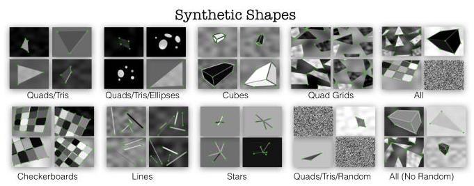
Figure 9. Synthetic Shapes Dataset. The Synthetic Shapes dataset consists of rendered triangles, quadrilaterals, lines, cubes, checkerboards, and stars each with ground truth corner locations. It also includes some negative images with no ground truth corners, such as ellipses and random noise images.
图 9. 合成形状数据集。合成形状数据集由渲染的三角形、四边形、直线、立方体、棋盘格和星星组成,每个都有真实角点位置。它还包括一些没有真实角点的负样本图像,如椭圆和随机噪声图像。
| Metric | Noise | MagicPointL | MagicPointS | FAST | Harris | Shi |
| mAP | no noise | 0.979 | 0.980 | 0.405 | 0.678 | 0.686 |
| mAP | noise | 0.971 | 0.939 | 0.061 | 0.213 | 0.157 |
| MLE | no noise | 0.860 | 0.922 | 1.656 | 1.245 | 1.188 |
| MLE | noise | 1.012 | 1.078 | 1.766 | 1.409 | 1.383 |
Table 5. Synthetic Shapes Results Table. Reports the mean Average Precision (mAP, higher is better) and Mean Localization Error (MLE, lower is better) across the 10 categories of images on the Synthetic Shapes dataset. Note that MagicPointL and Magic-PointS are relatively unaffected by imaging noise.
表5. 合成形状结果表。报告了合成形状数据集上10类图像的平均精度均值(mAP,越高越好)和平均定位误差(MLE,越低越好)。请注意,MagicPointL和Magic - PointS相对不受成像噪声的影响。
Mean Average Precision and Mean Localization Error. For each category, there are 1000 images sampled from the Synthetic Shapes generator. We compute Average Precision and Localization Error with and without added imaging noise. A summary of the per category results are shown in Figure 10 and the mean results are shown in Table 5. The MagicPoint detectors outperform the classical detectors in all categories. There is a significant performance gap in mAP in all categories in the presence of noise.
平均精度均值和平均定位误差。对于每个类别,从合成形状生成器中采样1000张图像。我们分别计算添加和不添加成像噪声时的平均精度和定位误差。每个类别的结果总结如图10所示,均值结果如表5所示。MagicPoint检测器在所有类别中都优于传统检测器。在有噪声的情况下,所有类别在mAP上都存在显著的性能差距。
Effect of Noise Magnitude. Next we study the effect of noise more carefully by varying its magnitude. We were curious if the noise we add to the images is too extreme and unreasonable for a point detector. To test this hypothesis, we linearly interpolate between the clean image \(\left( {s = 0}\right)\) and the noisy image \(\left( {s = 1}\right)\) . To push the detectors to the extreme, we also interpolate between the noisy image and random noise \(\left( {s = 2}\right)\) . The random noise images contain no geometric shapes, and thus produce an mAP score of 0.0 for all detectors. An example of the varying degree of noise and the plots are shown in Figure 11.
噪声幅度的影响。接下来,我们通过改变噪声幅度来更仔细地研究噪声的影响。我们好奇添加到图像中的噪声对于点检测器来说是否过于极端和不合理。为了验证这一假设,我们在干净图像 \(\left( {s = 0}\right)\) 和有噪声的图像 \(\left( {s = 1}\right)\) 之间进行线性插值。为了将检测器推向极限,我们还在有噪声的图像和随机噪声 \(\left( {s = 2}\right)\) 之间进行插值。随机噪声图像不包含几何形状,因此所有检测器的mAP分数均为0.0。不同噪声程度的示例和图表如图11所示。
Effect of Noise Type. We categorize the noise into eight categories. We study the effect of these noise types individually to better understand which has the biggest effect on the point detectors. Speckle noise is particularly difficult for traditional detectors. Results are summarized in Figure 12.
噪声类型的影响。我们将噪声分为八类。我们分别研究这些噪声类型的影响,以更好地了解哪种噪声对点检测器的影响最大。斑点噪声对传统检测器来说尤其困难。结果总结如图12所示。
Blob Detection. We experimented with our model's ability to detect the centers of shapes such as quadrilaterals and ellipses. We used the MagicPointL architecture (as described above) and augmented the Synthetic Shapes training set to include blob centers in addition to corners. We observed that our model was able to detect such blobs as long as the entire shape was not too large. However, the confidences produced for such "blob detection" are typically lower than those for corners, making it somewhat cumbersome to integrate both kinds of detections into a single system. For the main experiments in the paper, we omit training with blobs, except the following experiment.
斑点检测。我们测试了我们的模型检测四边形和椭圆等形状中心的能力。我们使用了MagicPointL架构(如上所述),并扩充了合成形状训练集,使其除了角点之外还包括斑点中心。我们观察到,只要整个形状不是太大,我们的模型就能检测到这样的斑点。然而,这种“斑点检测”产生的置信度通常低于角点检测的置信度,这使得将两种检测集成到一个系统中有些麻烦。在本文的主要实验中,我们省略了对斑点的训练,除了以下实验。
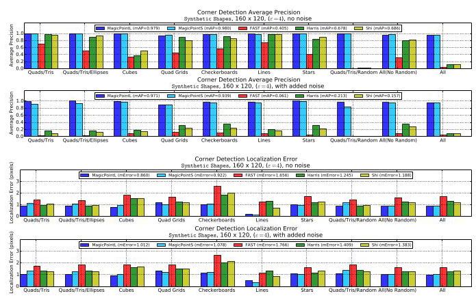
Figure 10. Per Shape Category Results. These plots report Average Precision and Corner Localization Error for each of the 10 categories in the Synthetic Shapes dataset with and without noise. The sequences with "Random" inputs are especially difficult for the classical detectors.
图10. 每个形状类别的结果。这些图表报告了合成形状数据集中10个类别在有噪声和无噪声情况下的平均精度和角点定位误差。具有“随机”输入的序列对传统检测器来说尤其困难。
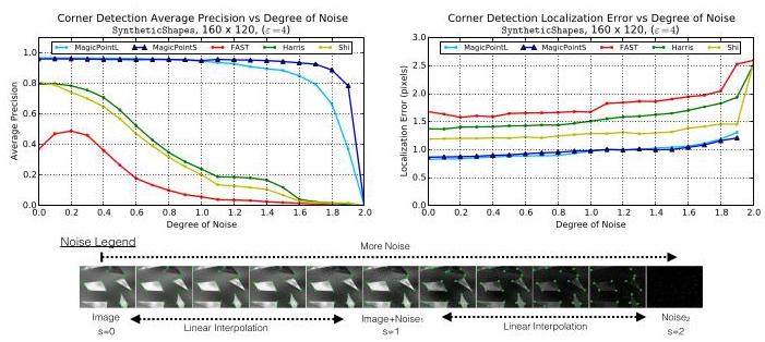
Figure 11. Effect of Noise Magnitude. Two versions of Magic-Point are compared to three classical point detectors on the Synthetic Shapes dataset (shown in Figure 9). The MagicPoint models outperform the classical techniques in both metrics, especially in the presence of image noise.
图11. 噪声幅度的影响。在合成形状数据集(如图9所示)上,将两种版本的Magic - Point与三种传统点检测器进行了比较。MagicPoint模型在两个指标上都优于传统技术,尤其是在存在图像噪声的情况下。
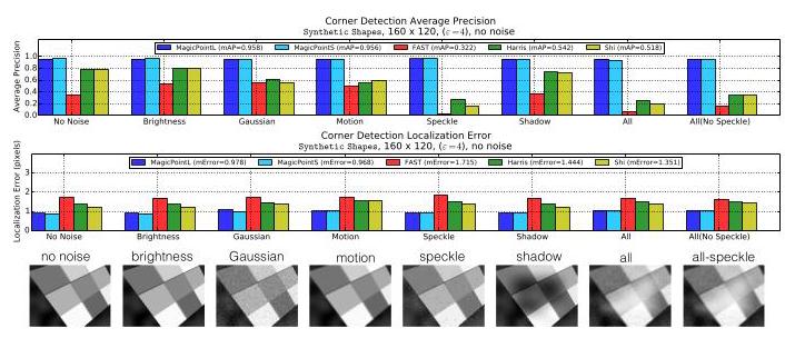
Figure 12. Effect of Noise Type. The detector performance is broken down by noise category. Speckle noise is particularly difficult for traditional detectors.
图12. 噪声类型的影响。检测器的性能按噪声类别进行了细分。斑点噪声对传统检测器来说尤其困难。
We created a sequence of \({96} \times {96}\) images of a black square on a white background. We vary the square's width to range from 3 to 91 pixels and report MagicPoint's confidence for two special pixels in the output heatmap: the center pixel (location of the blob) and the square's top-left pixel (an easy-to-detect corner). The MagicPoint blob+corner confidence plot for this experiment can be seen in Figure 13. We observe that we can confidently detect the center of the blob when the square is between 11 and 43 pixels wide (red region in Figure 13), detect with lower confidence when the square is between 43 and 71 pixels wide (yellow region in Figure 13), and unable to detect the center blob when the square is larger than 71 (blue regions in Figure 13).
我们创建了一系列 \({96} \times {96}\) 白色背景上黑色正方形的图像。我们将正方形的宽度从3像素变化到91像素,并报告MagicPoint在输出热图中两个特殊像素的置信度:中心像素(斑点位置)和正方形的左上角像素(易于检测的角点)。该实验的MagicPoint斑点 + 角点置信度图如图13所示。我们观察到,当正方形宽度在11到43像素之间时(图13中的红色区域),我们可以自信地检测到斑点的中心;当正方形宽度在43到71像素之间时(图13中的黄色区域),检测置信度较低;当正方形宽度大于71像素时(图13中的蓝色区域),无法检测到中心斑点。
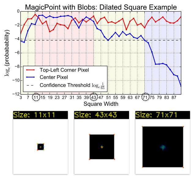
Figure 13. MagicPoint: Blob Center Detection Top: we experimented with MagicPoint's ability to detect the centers of shapes and plot detection confidences for both the top-left (TL) corner and the center blob. Bottom: point detection heatmaps (MagicPoint outputs) superimposed on the black rectangle images. Notice that our model is able to detect centers of 71 pixel rectangles, meaning that our network's receptive field is at least 71 pixels.
图13. MagicPoint:斑点中心检测 顶部:我们测试了MagicPoint检测形状中心的能力,并绘制了左上角(TL)角点和中心斑点的检测置信度。底部:点检测热图(MagicPoint输出)叠加在黑色矩形图像上。请注意,我们的模型能够检测71像素矩形的中心,这意味着我们网络的感受野至少为71像素。
C. Homographic Adaptation Experiment
C. 单应性自适应实验
When combining interest point response maps, it is important to differentiate between within-scale aggregation and across-scale aggregation. Real-world images typically contain features at different scales, as some points which would be deemed interesting in a high-resolution images, are often not even visible in coarser, lower resolution images. However, within a single-scale, transformations of the image such as rotations and translations should not make interest points appear/disappear. This underlying multi-scale nature of images has different implications for within-scale and across-scale aggregation strategies. Within-scale aggregation should be similar to computing the intersection of a set and across-scale aggregation should be similar to the union of a set. In other words, it is the average response within-scale that we really want, and the maximum response across-scale. We can additionally use the average response across scale as a multi-scale measure of interest point confidence. The average response across scales will be maximized when the interest point is visible across all scales, and these are likely to be the most robust interest points for tracking applications.
在组合兴趣点响应图时,区分尺度内聚合和跨尺度聚合非常重要。现实世界的图像通常包含不同尺度的特征,因为在高分辨率图像中被认为是有趣的一些点,在较粗糙、分辨率较低的图像中往往甚至不可见。然而,在单一尺度内,图像的旋转和平移等变换不应使兴趣点出现或消失。图像的这种潜在多尺度性质对尺度内和跨尺度聚合策略有不同的影响。尺度内聚合应类似于计算集合的交集,而跨尺度聚合应类似于计算集合的并集。换句话说,我们真正想要的是尺度内的平均响应,以及跨尺度的最大响应。我们还可以使用跨尺度的平均响应作为兴趣点置信度的多尺度度量。当兴趣点在所有尺度上都可见时,跨尺度的平均响应将达到最大值,而这些兴趣点可能是跟踪应用中最稳健的兴趣点。
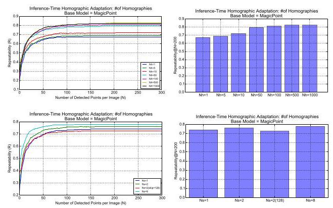
Figure 14. Homographic Adaptation. Top: we vary the number of homographies applied during Homographic Adaptation and report repeatability. Bottom: we isolate the effect of scale.
图14. 单应性自适应。顶部:我们改变单应性自适应过程中应用的单应性变换的数量,并报告重复性。底部:我们分离出尺度的影响。
Within-scale aggregation. We use the average response across a large number of Homographic warps of the input image. Care should be taken in choosing random homo-graphies because not all homographies are realistic image transformations. The number of homographic warps \({N}_{h}\) is a hyper-parameter of our approach. We typically enforce the first homography to be equal to identity, so that \({N}_{h} = 1\) in our experiments corresponds to doing no homographies (or equivalently, applying the identity Homography). Our experiments range from "small" \({N}_{h} = {10}\) , to "medium" \({N}_{h} = {100}\) , and "large" \({N}_{h} = {1000}\) .
尺度内聚合。我们使用输入图像大量单应性变换后的平均响应。在选择随机单应性变换时应谨慎,因为并非所有单应性变换都是现实的图像变换。单应性变换的数量 \({N}_{h}\) 是我们方法的一个超参数。我们通常强制第一个单应性变换为恒等变换,因此在我们的实验中 \({N}_{h} = 1\) 对应于不进行单应性变换(或者等效地,应用恒等单应性变换)。我们的实验范围从“小” \({N}_{h} = {10}\) 到“中” \({N}_{h} = {100}\) 以及“大” \({N}_{h} = {1000}\) 。
Across-scale aggregation. When aggregating across scales, the number of scales considered \({N}_{s}\) is a hyper-parameter of our approach. The setting of \({N}_{s} = 1\) corresponds to no multi-scale aggregation (or simply aggregating across the large possible image size only). For \({N}_{s} > 1\) , we refer to the multi-scale set of images being processed as "the multi-scale image pyramid." We consider weighting schemes that weigh levels of the pyramid differently, giving higher-resolution images a larger weight. This is important because interest points detected at lower resolutions have poorer localization ability, and we want the final aggregated points to be localized as well as possible.
跨尺度聚合。在进行跨尺度聚合时,考虑的尺度数量 \({N}_{s}\) 是我们方法的一个超参数。\({N}_{s} = 1\) 的设置对应于不进行多尺度聚合(或者简单地仅在最大可能的图像尺寸上进行聚合)。对于 \({N}_{s} > 1\) ,我们将正在处理的多尺度图像集称为“多尺度图像金字塔”。我们考虑采用不同的加权方案对金字塔的不同层级进行加权,给予高分辨率图像更大的权重。这很重要,因为在低分辨率下检测到的兴趣点的定位能力较差,我们希望最终聚合的点尽可能定位准确。
We experimented with within-scale and across-scale aggregation on a held out test of MS-COCO images. The results are summarized in Figure 14. We find that within-scale aggregation has the biggest effect on repeatability.
我们在MS - COCO图像的保留测试集上对尺度内和跨尺度聚合进行了实验。结果总结在图14中。我们发现尺度内聚合对重复性的影响最大。
D. Extra Qualitative Examples
D. 额外的定性示例
We show extra qualitative examples of SuperPoint, LIFT, SIFT and ORB on HPatches matching in Figure 15.
我们在图15中展示了SuperPoint、LIFT、SIFT和ORB在HPatches匹配上的额外定性示例。
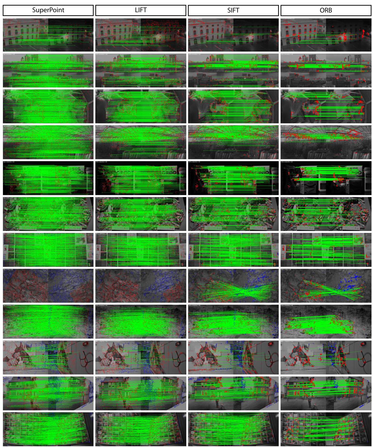
Figure 15. Extra Qualitative Results on HPatches. More examples like in Figure 8. The green lines show correct correspondences, green dots show matched points, red dots show mis-matched points, blue dots show points outside of the shared viewpoint region.
图15. HPatches上的额外定性结果。与图8类似的更多示例。绿色线条表示正确的对应关系,绿色圆点表示匹配的点,红色圆点表示不匹配的点,蓝色圆点表示共享视点区域外的点。

 浙公网安备 33010602011771号