sparkSQL的执行流程

spark sql 执行的流程图：

 

 

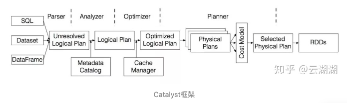
1. SQL 语句经过 SqlParser 解析成 Unresolved LogicalPlan;
2. 使用 analyzer 结合数据数据字典 (catalog) 进行绑定, 生成 resolved LogicalPlan;
3. 使用 optimizer 对 resolved LogicalPlan 进行优化, 生成 optimized LogicalPlan;
4. 使用 SparkPlan 将 LogicalPlan 转换成 PhysicalPlan;
5. 使用 prepareForExecution() 将 PhysicalPlan 转换成可执行物理计划;
6. 使用 execute() 执行可执行物理计划;
7. 生成 RDD

 分析spark sql的执行流程之前，可以先编译一下spark的源码，然后通过源码里面的examples工程做debug跟进，比只看源码要好很多

编译源码：https://segmentfault.com/a/1190000022723251

我这里使用的是spark 2.4.6版本

在spark的examples工程：org.apache.spark.examples.sql.SparkSQLExample

有一些sql，是可以帮助我们全程debug的

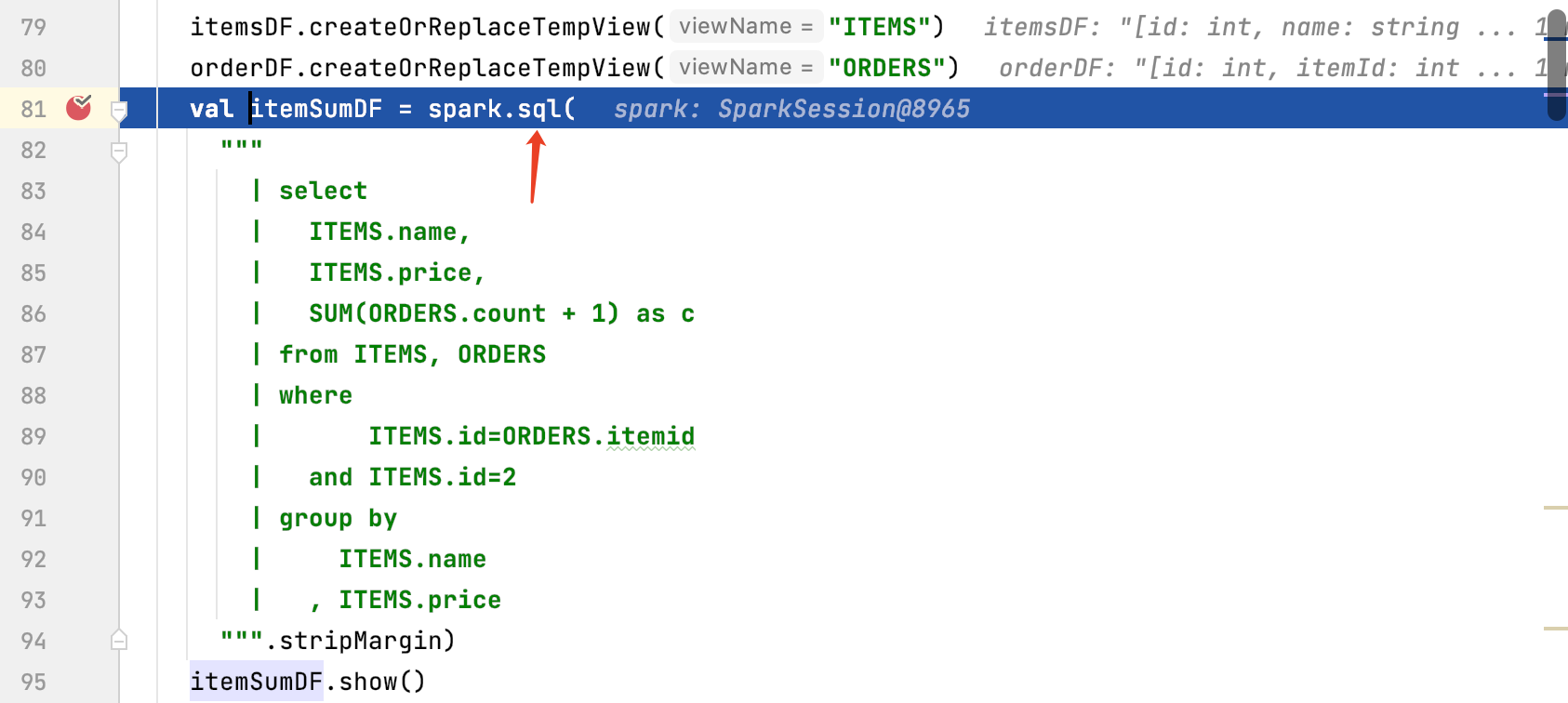
1、前期准备

val itemsDF = spark.createDataFrame(List(
      Item(1, "iphone 12 pro max", 12000)
      , Item(2, "iphone 11 pro max", 10500)
      , Item(3, "iphone X pro max", 9500)
    ))
    val orderDF = spark.createDataFrame(List(
      Order(100, 1, 2)
      , Order(101, 2, 4)
      , Order(102, 3, 2)

    ))
    itemsDF.createOrReplaceTempView("ITEMS")
    orderDF.createOrReplaceTempView("ORDERS")
    val itemSumDF = spark.sql(
      """
        | select
        |   ITEMS.name,
        |   ITEMS.price,
        |   SUM(ORDERS.count + 1) as c
        | from ITEMS, ORDERS
        | where
        |       ITEMS.id=ORDERS.itemid
        |   and ITEMS.id=2
        | group by
        |     ITEMS.name
        |   , ITEMS.price
      """.stripMargin)
    itemSumDF.show()

这里有兴趣的同学可以关注下：spark.createDataFrame 是如何将schema和数据进行捆绑的

2、词法解析

spark sql接收到sql后，需要通过antlr4进行词法和语法的解析。然后将sql文本根据antlr4的规则文件：SqlBase.g4 里面的规则进行逻辑解析

得到UnResolved Logical Plan 

代码是从spark.sql开始的：

 

 

当前这个解析的过程是由spark的catalyst工程完成的，主要是基于规则进行词法、语法解析，并对语法树基于规则和基于成本的优化。

Catalyst的核心是使用一个通用库生成树并使用规则操作这些树。在该框架的基础上，构建了用于关系查询处理库（例如表达式，逻辑查询计划）和处理执行查询不同阶段的几组规则：分析、逻辑优化、物理计划和代码生成，代码生成将部分查询编译为Java字节码。对于后者，使用了Scala特性quasiquotes，它可以很容易地在运行时由组合表达式生成代码

进入spark.sql的api

 

 

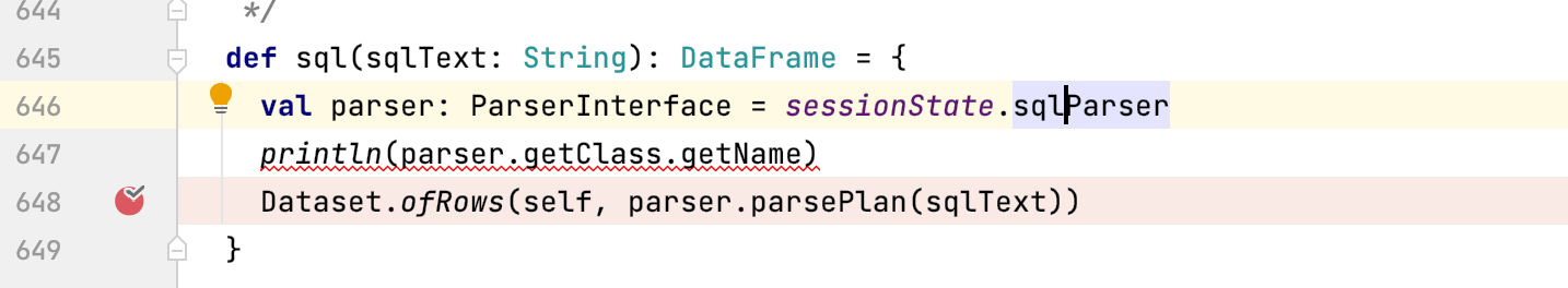
 里面ParserInterfance的实现类是：AbstractSqlParser ， 然后调用AbstractSqlParser.parsePlan

这里就需要进行词法和语法的解析，使用到了antlr：

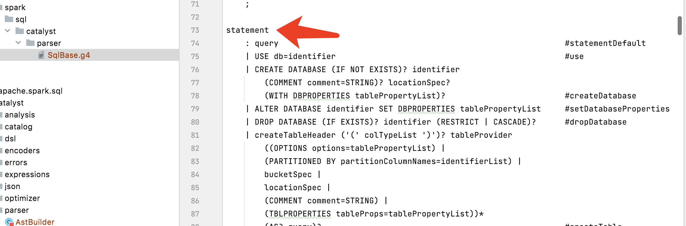
antlr4的使用需要定义一个语法文件，sparksql的语法文件的路径在sql/catalyst/src/main/antlr4/org/apache/spark/sql/catalyst/parser/SqlBase.g4 antlr可以使用插件自动生成词法解析和语法解析代码，在SparkSQL中词法解析器SqlBaseLexer和语法解析器SqlBaseParser，遍历节点有两种模式Listener和Visitor。

Listener模式是被动式遍历，antlr生成类ParseTreeListener，这个类里面包含了所有进入语法树中每个节点和退出每个节点时要进行的操作。我们只需要实现我们需要的节点事件逻辑代码即可，再实例化一个遍历类ParseTreeWalker，antlr会自上而下的遍历所有节点，以完成我们的逻辑处理；

Visitor则是主动遍历模式，需要我们显示的控制我们的遍历顺序。该模式可以实现在不改变各元素的类的前提下定义作用于这些元素的新操作。SparkSql用的就是此方式来遍历节点的。

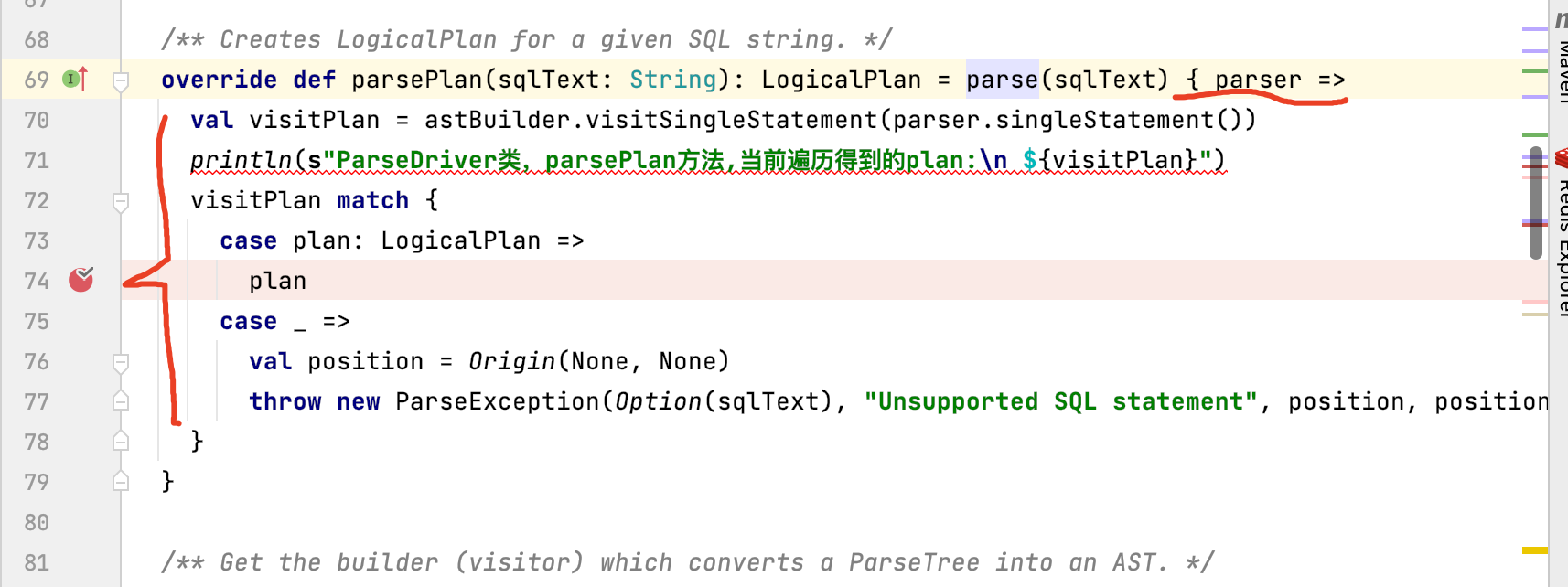
通过词法解析和语法解析将SQL语句解析成了ANTLR 4的语法树结构ParseTree。然后在parsePlan中，使用AstBuilder将ANTLR 4语法树结构转换成catalyst表达式逻辑计划logical plan

这个方法首先对sql进行词法和语法的解析：parse(sqlText) ， 然后通过Ast语法树进行遍历。可以看到是通过visit的模式，遍历SingleStatement，就是antlr文件的入口规则

SingleStatementContext是整个抽象语法树的根节点，因此以AstBuilder的visitSingleStatement方法为入口来遍历抽象语法树

 

 

 antlr4的规则入口：

 

 

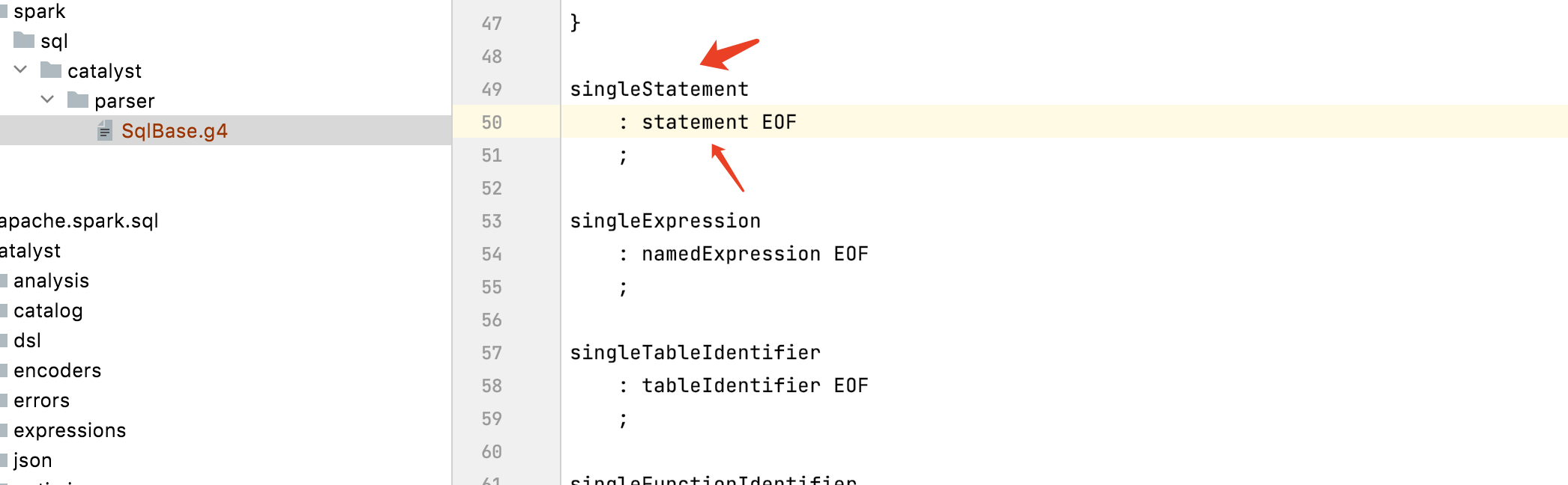
下面就是匹配整个spark sql语法的逻辑 

 

 

 其中词法和语法的解析代码是：

parse(sqlText)

根据java的代码重写规则，其实是：

SparkSqlParser#parse

仔细观察不难发现当前的parse方法是一个柯里化

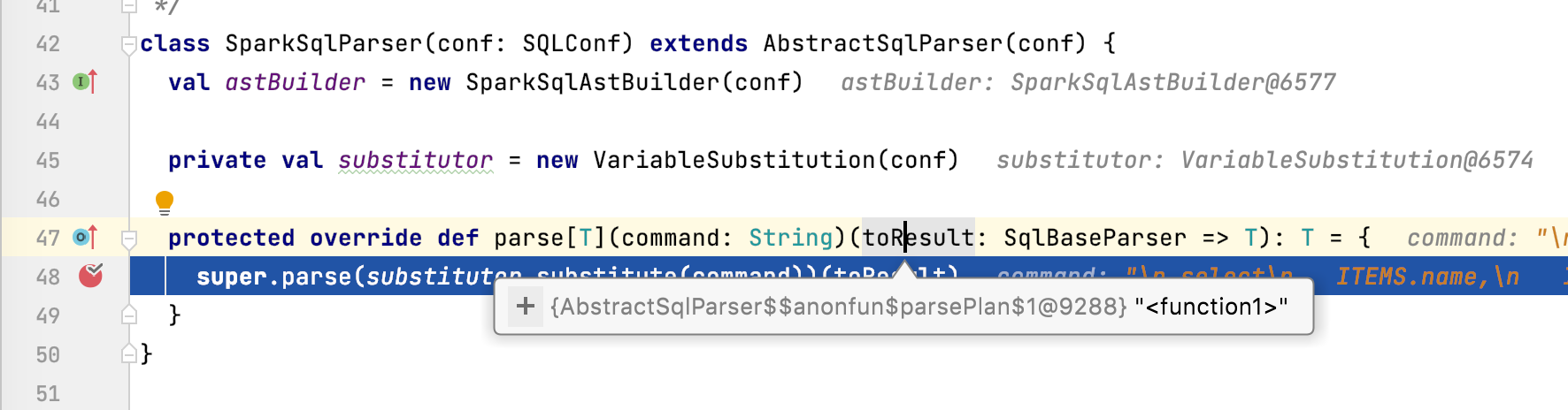
 这样程序会调用到当前SparkSqlParser的父类:

AbstractSqlParser#parsePlan

当前方法主要做以下3件事：

1、将sql变成字节流的方式，传入词法解析器上

2、根据词法解析产生的Token序列进行语法解析

3、执行柯里化的方法

 

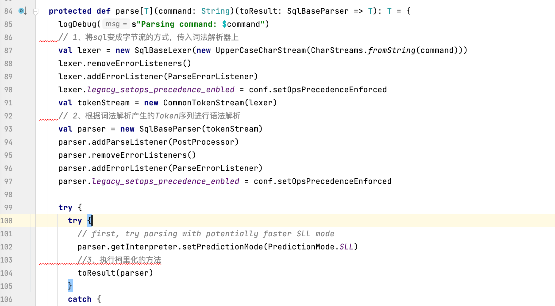
这个柯里化代码的实现就是上一步的匿名函数：

3、语法解析

所以当词法和语法解析结束后，就会进入这个柯里化。

当前的柯里化主要做如下2件事：

1、通过visit的模式主动遍历(递归) UnResolved Logical Plan 

2、得到遍历后的结果，按照模式匹配方式，将结果返回

其中遍历，其实就是根据解析后的UnResolved Logical Plan 结构，参照SqlBase.g4的语法树进行匹配

比如，我这里的sql是：

select
   ITEMS.name,
   ITEMS.price,
   SUM(ORDERS.count + 1) as c
 from ITEMS, ORDERS
 where
       ITEMS.id=ORDERS.itemid
   and ITEMS.id=2
 group by
     ITEMS.name
   , ITEMS.price
      

那么解析出来的UnResolved Logical Plan结构就是：

'Aggregate ['ITEMS.name, 'ITEMS.price], ['ITEMS.name, 'ITEMS.price, 'SUM(('ORDERS.count + 1)) AS c#12]
+- 'Filter (('ITEMS.id = 'ORDERS.itemid) && ('ITEMS.id = 2))
   +- 'Join Inner
      :- 'UnresolvedRelation `ITEMS`
      +- 'UnresolvedRelation `ORDERS`

 

值得注意的是，当前解析出来的数据源结构是：UnresolvedRelation

这种结构是还没有跟catalog建立关联关系的类，详细可以参考：https://blog.csdn.net/qq_41775852/article/details/105189828

这样当前得到了unResolved的语法树，然后程序就进入到：

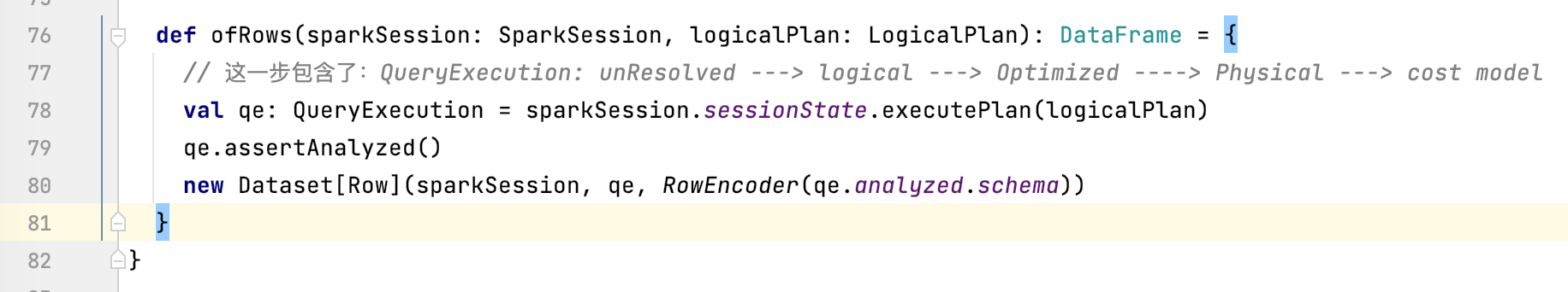
Dataset.ofRows(self, parser.parsePlan(sqlText))

Dataset.ofRows这一步包含了：

1、构建QueryExecution

2、QueryExecution: unResolved ---> logical ---> Optimized ----> Physical ---> cost model

 

首先通过以下代码，将语法树转化如下结构的过程：unResolved ---> logical ---> Optimized ----> Physical

val qe: QueryExecution = sparkSession.sessionState.executePlan(logicalPlan)

qe.assertAnalyzed()

得到如下过程：

== Parsed Logical Plan ==
'Aggregate ['ITEMS.name, 'ITEMS.price], ['ITEMS.name, 'ITEMS.price, 'SUM(('ORDERS.count + 1)) AS c#12]
+- 'Filter (('ITEMS.id = 'ORDERS.itemid) && ('ITEMS.id = 2))
   +- 'Join Inner
      :- 'UnresolvedRelation `ITEMS`
      +- 'UnresolvedRelation `ORDERS`

== Analyzed Logical Plan ==
name: string, price: float, c: bigint
Aggregate [name#1, price#2], [name#1, price#2, sum(cast((count#8 + 1) as bigint)) AS c#12L]
+- Filter ((id#0 = itemid#7) && (id#0 = 2))
   +- Join Inner
      :- SubqueryAlias `items`
      :  +- LocalRelation [id#0, name#1, price#2]
      +- SubqueryAlias `orders`
         +- LocalRelation [id#6, itemId#7, count#8]

== Optimized Logical Plan ==
Aggregate [name#1, price#2], [name#1, price#2, sum(cast((count#8 + 1) as bigint)) AS c#12L]
+- Project [name#1, price#2, count#8]
   +- Join Inner, (id#0 = itemid#7)
      :- LocalRelation [id#0, name#1, price#2]
      +- LocalRelation [itemId#7, count#8]

== Physical Plan ==
*(2) HashAggregate(keys=[name#1, price#2], functions=[sum(cast((count#8 + 1) as bigint))], output=[name#1, price#2, c#12L])
+- Exchange hashpartitioning(name#1, price#2, 200)
   +- *(1) HashAggregate(keys=[name#1, price#2], functions=[partial_sum(cast((count#8 + 1) as bigint))], output=[name#1, price#2, sum#15L])
      +- *(1) Project [name#1, price#2, count#8]
         +- *(1) BroadcastHashJoin [id#0], [itemid#7], Inner, BuildRight
            :- LocalTableScan [id#0, name#1, price#2]
            +- BroadcastExchange HashedRelationBroadcastMode(List(cast(input[0, int, false] as bigint)))
               +- LocalTableScan [itemId#7, count#8]

上面打印出来的结果是在 QueryExecution的toString打印出来的；

== Parsed Logical Plan ==
就是在构造QueryExecution时候传入的LogicalPlan

== Analyzed Logical Plan ==
是通过QueryExecution#analyzed进行处理后得到的结果

== Optimized Logical Plan ==
是用过QueryExecution里面的

sparkSession.sessionState.optimizer.execute(withCachedData)得到的结果

lazy val optimizedPlan: LogicalPlan = sparkSession.sessionState.optimizer.execute(withCachedData)

== Physical Plan ==
是通过lazy val executedPlan: SparkPlan = prepareForExecution(sparkPlan)得到的结果

值得注意的事情是，QueryExecution里面这些关键函数都是lazy的，也就是初始化的时候并不会被调用，而是在被动调用的情况下才会触发

4、== Analyzed Logical Plan ==阶段

lazy val analyzed: LogicalPlan = {
    SparkSession.setActiveSession(sparkSession)
    val analyzer: Analyzer = sparkSession.sessionState.analyzer
    analyzer.executeAndCheck(logical)
  }

1、首先将父线程的sparksession变量传递到子线程（https://blog.csdn.net/hewenbo111/article/details/80487252）

2、然后获取构造函数传递来的analyzer

3、执行分析

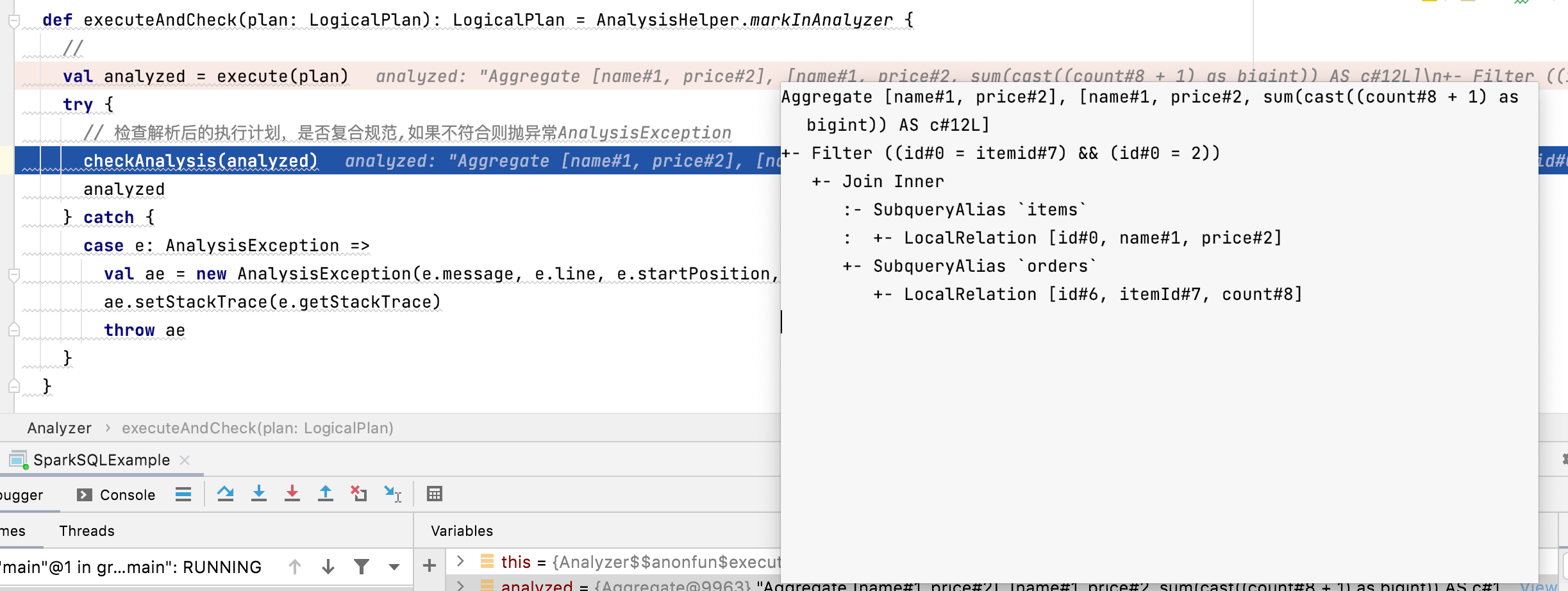
进入：analyzer.executeAndCheck(logical) 查看代码，逻辑是：

1、根据spark规定的一系列规则（batches）对语法树进行匹配，也就是规则解析，这一阶段会将Unresolved变成Resolved

2、然后检查规则解析后的LogicalPlan，是否复合规范

 

 跟进checkAnalysis(analyzed)，程序最终会走到RuleExecutor#execute方法

def execute(plan: TreeType): TreeType = {
    var curPlan = plan
    val queryExecutionMetrics = RuleExecutor.queryExecutionMeter
    /** batches是提前定义好的一些规则*/
    batches.foreach { batch =>
      val batchStartPlan = curPlan
      var iteration = 1
      var lastPlan = curPlan
      var continue = true

      // Run until fix point (or the max number of iterations as specified in the strategy.
      while (continue) {
        val rules: Seq[Rule[TreeType]] = batch.rules
        curPlan = rules.foldLeft(curPlan) { //进行规则匹配
          case (plan, rule) =>
            val startTime = System.nanoTime()
            val result = rule(plan) // 规则解析
            val runTime = System.nanoTime() - startTime

            if (!result.fastEquals(plan)) {
              queryExecutionMetrics.incNumEffectiveExecution(rule.ruleName)
              queryExecutionMetrics.incTimeEffectiveExecutionBy(rule.ruleName, runTime)
              logTrace(
                s"""
                  |=== Applying Rule ${rule.ruleName} ===
                  |${sideBySide(plan.treeString, result.treeString).mkString("\n")}
                """.stripMargin)
            }
            queryExecutionMetrics.incExecutionTimeBy(rule.ruleName, runTime)
            queryExecutionMetrics.incNumExecution(rule.ruleName)
            log.info("当前的规则名称为：{}" ,rule.ruleName)

            // Run the structural integrity checker against the plan after each rule.
            if (!isPlanIntegral(result)) {
              val message = s"After applying rule ${rule.ruleName} in batch ${batch.name}, " +
                "the structural integrity of the plan is broken."
              throw new TreeNodeException(result, message, null)
            }

            result
        }
        log.info("当前规则解析迭代次数是：{}" , iteration)
        iteration += 1
        if (iteration > batch.strategy.maxIterations) {
          // Only log if this is a rule that is supposed to run more than once.
          if (iteration != 2) {
            val message = s"Max iterations (${iteration - 1}) reached for batch ${batch.name}"
            if (Utils.isTesting) {
              throw new TreeNodeException(curPlan, message, null)
            } else {
              logWarning(message)
            }
          }
          continue = false
        }
        //如果当前batch下的全部rule都解析完毕，跳出while循环
        if (curPlan.fastEquals(lastPlan)) {
          logTrace(
            s"Fixed point reached for batch ${batch.name} after ${iteration - 1} iterations.")
          continue = false
        }
        lastPlan = curPlan
      }

      if (!batchStartPlan.fastEquals(curPlan)) {
        logDebug(
          s"""
            |=== Result of Batch ${batch.name} ===
            |${sideBySide(batchStartPlan.treeString, curPlan.treeString).mkString("\n")}
          """.stripMargin)
      } else {
        logTrace(s"Batch ${batch.name} has no effect.")
      }
    }

    curPlan
  }

期核心逻辑就是，程序在初始化Analysis类的时候，会初始化一些规则，然后根据这些规则来匹配执行计划，进行逻辑解析和优化一些工作

其中的规则是： 其中一些规则的功能参考地址:https://www.modb.pro/db/407250

lazy val batches: Seq[Batch] = Seq(
    Batch("Hints", fixedPoint,
      new ResolveHints.ResolveBroadcastHints(conf),
      ResolveHints.ResolveCoalesceHints,
      ResolveHints.RemoveAllHints),
    Batch("Simple Sanity Check", Once,
      LookupFunctions),
    Batch("Substitution", fixedPoint,
      CTESubstitution,
      WindowsSubstitution,
      EliminateUnions,
      new SubstituteUnresolvedOrdinals(conf)),
    Batch("Resolution", fixedPoint,
      ResolveTableValuedFunctions ::
      ResolveRelations ::
      ResolveReferences ::
      ResolveCreateNamedStruct ::
      ResolveDeserializer ::
      ResolveNewInstance ::
      ResolveUpCast ::
      ResolveGroupingAnalytics ::
      ResolvePivot ::
      ResolveOrdinalInOrderByAndGroupBy ::
      ResolveAggAliasInGroupBy ::
      ResolveMissingReferences ::
      ExtractGenerator ::
      ResolveGenerate ::
      ResolveFunctions ::
      ResolveAliases ::
      ResolveSubquery ::
      ResolveSubqueryColumnAliases ::
      ResolveWindowOrder ::
      ResolveWindowFrame ::
      ResolveNaturalAndUsingJoin ::
      ResolveOutputRelation ::
      ExtractWindowExpressions ::
      GlobalAggregates ::
      ResolveAggregateFunctions ::
      TimeWindowing ::
      ResolveInlineTables(conf) ::
      ResolveHigherOrderFunctions(catalog) ::
      ResolveLambdaVariables(conf) ::
      ResolveTimeZone(conf) ::
      ResolveRandomSeed ::
      TypeCoercion.typeCoercionRules(conf) ++
      extendedResolutionRules : _*),
    Batch("Post-Hoc Resolution", Once, postHocResolutionRules: _*),
    Batch("Nondeterministic", Once,
      PullOutNondeterministic),
    Batch("UDF", Once,
      HandleNullInputsForUDF),
    Batch("FixNullability", Once,
      FixNullability),
    Batch("Subquery", Once,
      UpdateOuterReferences),
    Batch("Cleanup", fixedPoint,
      CleanupAliases)
  )

这个Batch可以翻译过来称为逻辑计划执行策略组更容易理解一些。里面包含了针对每一类别LogicalPlan的处理类。每个Batch需要指定其名称、执行策略、以及规则。

经过上述的规则解析之后，就会把之前的UnresolvedRelation 解析出来

== Parsed Logical Plan ==
'Aggregate ['ITEMS.name, 'ITEMS.price], ['ITEMS.name, 'ITEMS.price, 'SUM(('ORDERS.count + 1)) AS c#12]
+- 'Filter (('ITEMS.id = 'ORDERS.itemid) && ('ITEMS.id = 2))
   +- 'Join Inner
      :- 'UnresolvedRelation `ITEMS`
      +- 'UnresolvedRelation `ORDERS`

== Analyzed Logical Plan ==
name: string, price: float, c: bigint
Aggregate [name#1, price#2], [name#1, price#2, sum(cast((count#8 + 1) as bigint)) AS c#12L]
+- Filter ((id#0 = itemid#7) && (id#0 = 2))
   +- Join Inner
      :- SubqueryAlias `items`
      :  +- LocalRelation [id#0, name#1, price#2]
      +- SubqueryAlias `orders`
         +- LocalRelation [id#6, itemId#7, count#8]

 

 然后进行检查当前解析后的执行计划是否复合规范。到此为止就是将未解析的执行计划变成解析后的执行计划。但是看执行计划还是有优化的地方

1、比如在sum的时候存在常量的加法操作（这样会导致每条数据都要加法一次，数据量大的话会浪费CPU）

2、如果当前的表比较小，那么应该是BroadCastJoin优于当前的inner join  

所以到这里程序并没有接续，接下来要做的是Optimized Logical Plan

5、== Optimized Logical Plan ==

spark sql经过

== Parsed Logical Plan == 和 == Analyzed Logical Plan ==两步骤后，就已经将元数据信息与catalog进行了绑定

然后代码会调用：

lazy val optimizedPlan: LogicalPlan = sparkSession.sessionState.optimizer.execute(withCachedData)

然后流程跟Analysis一样，程序进入RuleExecutor#execute。不一样的是当前的batches是Optimizer里面的defaultBatches和sparkOptimer里面的defaultBatches

Optimizer里面的defaultBatches

  /**
   * Defines the default rule batches in the Optimizer.
   *
   * Implementations of this class should override this method, and [[nonExcludableRules]] if
   * necessary, instead of [[batches]]. The rule batches that eventually run in the Optimizer,
   * i.e., returned by [[batches]], will be (defaultBatches - (excludedRules - nonExcludableRules)).
   */
  def defaultBatches: Seq[Batch] = {
    val operatorOptimizationRuleSet =
      Seq(
        // Operator push down
        PushProjectionThroughUnion, // 对于全部是确定性 Project 进行下推
        ReorderJoin, // 根据 Join 关联条件，进行顺序重排
        EliminateOuterJoin, // 消除非空约束的 Outer Join
        PushDownPredicates, // 谓词下推
        PushDownLeftSemiAntiJoin, // Project、Window、Union、Aggregate、PushPredicateThroughNonJoin 场景下，下推 LeftSemi/LeftAnti
        PushLeftSemiLeftAntiThroughJoin, // Join 场景下，下推 LeftSemi/LeftAnti
        LimitPushDown, // Limit 下推
        ColumnPruning, // 列裁剪
        InferFiltersFromConstraints, // 根据约束推断 Filter 信息
        // Operator combine
        CollapseRepartition, // 合并 Repartition
        CollapseProject, // 合并 Project
        CollapseWindow, // 合并 Window（相同的分区及排序）
        CombineFilters, // 合并 Filter
        CombineLimits, // 合并 Limit
        CombineUnions, // 合并 Union
        // Constant folding and strength reduction
        TransposeWindow, // 转置 Window，优化计算
        NullPropagation, // Null 传递
        ConstantPropagation, // 常量传递
        FoldablePropagation, // 可折叠字段、属性传播
        OptimizeIn, // 优化 In，空处理、重复处理
        ConstantFolding, // 常量折叠
        ReorderAssociativeOperator, // 排序与折叠变量
        LikeSimplification, // 优化 Like 对应的正则
        BooleanSimplification, // 简化 Boolean 表达式
        SimplifyConditionals, // 简化条件表达式，if/case
        RemoveDispensableExpressions, // 移除不必要的节点，positive
        SimplifyBinaryComparison, // 优化比较表达式为 Boolean Literal
        ReplaceNullWithFalseInPredicate, // 优化 Null 场景 Literal
        PruneFilters, // 裁剪明确的过滤条件
        EliminateSorts, // 消除 Sort，无关或重复
        SimplifyCasts, // 简化 Cast，类型匹配
        SimplifyCaseConversionExpressions, // 简化 叠加的大小写转换
        RewriteCorrelatedScalarSubquery, // 子查询改写为 Join
        EliminateSerialization, // 消除 序列化
        RemoveRedundantAliases, // 删除冗余的别名
        RemoveNoopOperators, // 删除没有操作的操作符
        SimplifyExtractValueOps, // 简化符合类型操作符
        CombineConcats) ++ // 合并 Concat 表达式
        extendedOperatorOptimizationRules // 扩展规则

    val operatorOptimizationBatch: Seq[Batch] = {
      val rulesWithoutInferFiltersFromConstraints =
        operatorOptimizationRuleSet.filterNot(_ == InferFiltersFromConstraints)
      Batch("Operator Optimization before Inferring Filters", fixedPoint,
        rulesWithoutInferFiltersFromConstraints: _*) ::
      Batch("Infer Filters", Once,
        InferFiltersFromConstraints) ::
      Batch("Operator Optimization after Inferring Filters", fixedPoint,
        rulesWithoutInferFiltersFromConstraints: _*) :: Nil
    }

    (Batch("Eliminate Distinct", Once, EliminateDistinct) :: // 消除聚合中冗余的 Distinct
    // Technically some of the rules in Finish Analysis are not optimizer rules and belong more
    // in the analyzer, because they are needed for correctness (e.g. ComputeCurrentTime).
    // However, because we also use the analyzer to canonicalized queries (for view definition),
    // we do not eliminate subqueries or compute current time in the analyzer.
    Batch("Finish Analysis", Once,
      EliminateResolvedHint, // 通过 Join 改写 Hint
      EliminateSubqueryAliases, // 消除 子查询别名
      EliminateView, // 消除 视图
      ReplaceExpressions, // 替换、改写 表达式
      ComputeCurrentTime, // 计算当前日期或时间
      GetCurrentDatabase(sessionCatalog), // 替换当前的数据库
      RewriteDistinctAggregates, // Distinct 优化改写
      ReplaceDeduplicateWithAggregate) :: // 通过聚合优化删除重复数据算子
    //////////////////////////////////////////////////////////////////////////////////////////
    // Optimizer rules start here
    //////////////////////////////////////////////////////////////////////////////////////////
    // - Do the first call of CombineUnions before starting the major Optimizer rules,
    //   since it can reduce the number of iteration and the other rules could add/move
    //   extra operators between two adjacent Union operators.
    // - Call CombineUnions again in Batch("Operator Optimizations"),
    //   since the other rules might make two separate Unions operators adjacent.
    Batch("Union", Once,
      CombineUnions) :: // 合并相邻的 Union
    Batch("OptimizeLimitZero", Once,
      OptimizeLimitZero) :: // 优化 limit 0
    // Run this once earlier. This might simplify the plan and reduce cost of optimizer.
    // For example, a query such as Filter(LocalRelation) would go through all the heavy
    // optimizer rules that are triggered when there is a filter
    // (e.g. InferFiltersFromConstraints). If we run this batch earlier, the query becomes just
    // LocalRelation and does not trigger many rules.
    Batch("LocalRelation early", fixedPoint,
      ConvertToLocalRelation, // 优化 LocalRelation
      PropagateEmptyRelation) :: // 优化 EmptyRelation
    Batch("Pullup Correlated Expressions", Once,
      PullupCorrelatedPredicates) :: // 处理引用外部谓词
    Batch("Subquery", Once,
      OptimizeSubqueries) :: // 优化 子查询，去除不必要排序
    Batch("Replace Operators", fixedPoint,
      RewriteExceptAll, // 重写 Except All
      RewriteIntersectAll, // 重写 Intersect All
      ReplaceIntersectWithSemiJoin, // 使用 Semi Join，重写 Intersect
      ReplaceExceptWithFilter, // 使用 Filter，重写 Except
      ReplaceExceptWithAntiJoin, // 使用 Anti Join，重写 Except
      ReplaceDistinctWithAggregate) :: // 使用 Aggregate，重写 Distinct
    Batch("Aggregate", fixedPoint,
      RemoveLiteralFromGroupExpressions, // 删除聚合表达式的字面量
      RemoveRepetitionFromGroupExpressions) :: Nil ++ // 删除聚合表达式的重复信息
    operatorOptimizationBatch) :+
    Batch("Join Reorder", Once,
      CostBasedJoinReorder) :+ // 基于损失的 Join 重排
    Batch("Remove Redundant Sorts", Once,
      RemoveRedundantSorts) :+ // 删除冗余的排序
    Batch("Decimal Optimizations", fixedPoint,
      DecimalAggregates) :+ // Decimal 类型聚合优化
    Batch("Object Expressions Optimization", fixedPoint,
      EliminateMapObjects, // 消除 MapObject
      CombineTypedFilters, // 合并相邻的类型过滤
      ObjectSerializerPruning, // 裁剪不必要的序列化
      ReassignLambdaVariableID) :+ // 重新分类 LambdaVariable ID，利于 codegen 优化
    Batch("LocalRelation", fixedPoint,
      ConvertToLocalRelation, // 优化 LocalRelation
      PropagateEmptyRelation) :+ // 优化 EmptyRelation
    Batch("Extract PythonUDF From JoinCondition", Once,
      PullOutPythonUDFInJoinCondition) :+ // 标识 Join 中的 PythonUDF
    // The following batch should be executed after batch "Join Reorder" "LocalRelation" and
    // "Extract PythonUDF From JoinCondition".
    Batch("Check Cartesian Products", Once,
      CheckCartesianProducts) :+ // 检测 笛卡尔积 约束条件
    Batch("RewriteSubquery", Once,
      RewritePredicateSubquery, // 重写 子查询，EXISTS/NOT EXISTS、IN/NOT IN
      ColumnPruning, // 裁剪列
      CollapseProject, // 合并投影
      RemoveNoopOperators) :+ // 删除无用的操作符
    // This batch must be executed after the `RewriteSubquery` batch, which creates joins.
    Batch("NormalizeFloatingNumbers", Once, NormalizeFloatingNumbers) // 规范 Float 类型数值
  }

 

SparkOptimer里面的defaultBatches、

override def defaultBatches: Seq[Batch] = (preOptimizationBatches ++ super.defaultBatches :+
    Batch("Optimize Metadata Only Query", Once, OptimizeMetadataOnlyQuery(catalog)) :+
    Batch("Extract Python UDFs", Once,
      Seq(ExtractPythonUDFFromAggregate, ExtractPythonUDFs): _*) :+
    Batch("Prune File Source Table Partitions", Once, PruneFileSourcePartitions) :+
    Batch("Parquet Schema Pruning", Once, ParquetSchemaPruning)) ++
    postHocOptimizationBatches :+
    Batch("User Provided Optimizers", fixedPoint, experimentalMethods.extraOptimizations: _*)

这样Analyzed Logical Plan经过Optimer里面的一些列规则匹配后，形成优化后的执行计划

5.1、优化规则1：Operator push down 优化下推操作

下推的优化规则有下面几种：(这些规则优化会有交叉)

PushProjectionThroughUnion,
ReorderJoin,
EliminateOuterJoin,
PushPredicateThroughJoin,
PushDownPredicate,
LimitPushDown,
ColumnPruning,
InferFiltersFromConstraints,

 

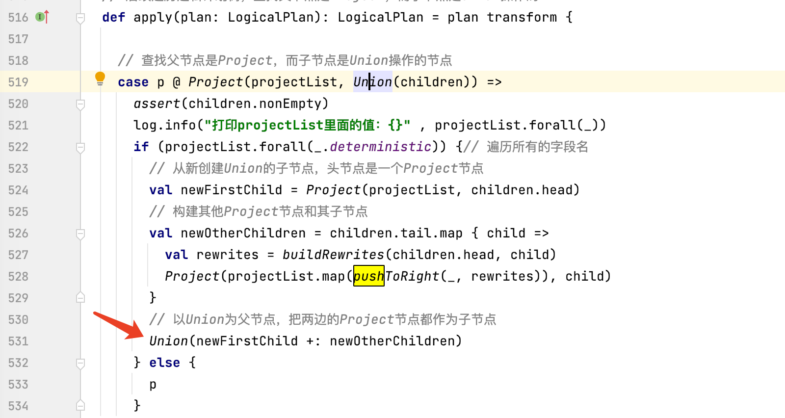
1、PushProjectionThroughUnion操作下推优化规则的作用是：把在Union操作一边的Projections（投影）操作推到Union的两边。 

要注意这样优化的前提是在Spark SQL中union操作不会对数据去重（union 和union all的区别）。

这里的Projections可以理解为select字段的操作。也就是说，把select操作推到Union操作的两边 

 

 

 

 

2、ReorderJoin：对Join操作进行重新排列，把所有的过滤条件推入join中，以便保证join内部至少有一个过滤条件。

3、EliminateOuterJoin：尽可能的消除outer join。在条件允许的情况下对outer join进行优化，尽可能消除和优化outer join，尽量使用其他join类型来代替，比如：inner join

4、PushPredicateThroughJoin ：

1.Join+where子句的实现逻辑
（1）若是Inner Join则把过滤条件下推到参加Join的两端
（2）若是 RightOuter，则把where子句的右侧数据集的过滤条件下推到右侧数据集。
（3）若是LeftOuter，则把where子句中左侧数据集的过滤条件下推到左侧数据集。
（4）若是FullOuter，则不会下推where子句的过滤条件到数据集。

2.Join+on子句的实现逻辑
（1）若是Inner Join把on子句的过滤条件下推到参加Join的两端的数据及中。
（2）若是RightOuter，把on子句中左侧数据集的过滤条件下推到左侧数据集中。
（3）若是LeftOuter，把on子句中右侧数据集的过滤条件下推到右侧数据集中。
（4）若是FullOuter，则不会下推on子句的过滤条件到数据集

 

5、PushDownPredicate

谓词下推，这个过程主要将过滤条件尽可能地下推到底层，最好是数据源

6、LimitPushDown

把limit操作进行下推，尽量下推到读取数据时。

另外，该规则还有一个限制条件，就是当union all、left outer join、right outer join操作 结合limit操作时才生效

 

 

 

7、ColumnPruning

列减枝操作。有时候查询sql类似：

select name from (select * from table) a

实际只需要一列name，但为了写方便，子查询查询了所有的列。这样会出现更大的IO成本

因此通过ColumnPruning可以在数据源处过滤掉不需要查询的列

8、InferFiltersFromConstraints

对Filter结点的约束条件进行分析，添加额外的过滤条件列表，比如经常在执行计划中看到isNotNull 实际我们并没有在sql中写，但是InferFiltersFromConstraints会帮我们生成一些额外的过滤条件

 

测试下推-谓词的下推：

表结构：

case class Item(id:Int, name:String, price:Float)
case class ItemTmp(id:Int, name:String, price:Float)

1、测试sql_1，验证对于

PushProjectionThroughUnion

PushDownPredicate

ColumnPruning

（使用union all）【如果使用union 则不会生效】

val itemSumDF = spark.sql(
      """
        |select id  from
        |(
        |select * from ITEMS
        |union all
        |select * from itemsTmpDF
        |) a
        |""".stripMargin)

 

场景1: 去掉Optimizer里面的对谓词的下推和列剪枝操作

PushProjectionThroughUnion
PushDownPredicate
ColumnPruning

得到的执行计划：

== Analyzed Logical Plan ==
id: int
Project [id#0]
+- Filter (id#0 > 2)
   +- SubqueryAlias `a`
      +- Union
         :- Project [id#0, name#1, price#2]
         :  +- SubqueryAlias `items`
         :     +- LocalRelation [id#0, name#1, price#2]
         +- Project [id#6, name#7, price#8]
            +- SubqueryAlias `itemstmpdf`
               +- LocalRelation [id#6, name#7, price#8]

== Optimized Logical Plan ==
Project [id#0]
+- Filter (id#0 > 2)
   +- Union
      :- Project [id#0]
      :  +- LocalRelation [id#0, name#1, price#2]
      +- Project [id#6]
         +- LocalRelation [id#6, name#7, price#8]

再把上面的操作添加上执行后，得到如下执行计划：

== Analyzed Logical Plan ==
id: int
Project [id#0]
+- Filter (id#0 > 2)
   +- SubqueryAlias `a`
      +- Union
         :- Project [id#0, name#1, price#2]
         :  +- SubqueryAlias `items`
         :     +- LocalRelation [id#0, name#1, price#2]
         +- Project [id#6, name#7, price#8]
            +- SubqueryAlias `itemstmpdf`
               +- LocalRelation [id#6, name#7, price#8]

== Optimized Logical Plan ==
Union
:- LocalRelation [id#0]
+- LocalRelation [id#6]

 

场景2：验证PushPredicateThroughJoin规则

表结构

case class Item(id:Int, name:String, price:Float)
case class Order(id:Int, itemId:Int, count:Int)

sql：

select
   ITEMS.name,
   ITEMS.price
 from
 ITEMS left join ORDERS
 on ITEMS.id=ORDERS.itemid
 where ITEMS.id=2 and ORDERS.itemid > 1 and ITEMS.price > 0

 

再去掉优化规则：PushPredicateThroughJoin，得到的执行计划：

== Analyzed Logical Plan ==
name: string, price: float
Project [name#1, price#2]
+- Filter (((id#0 = 2) && (itemid#13 > 1)) && (price#2 > cast(0 as float)))
   +- Join LeftOuter, (id#0 = itemid#13)
      :- SubqueryAlias `items`
      :  +- LocalRelation [id#0, name#1, price#2]
      +- SubqueryAlias `orders`
         +- LocalRelation [id#12, itemId#13, count#14]

== Optimized Logical Plan ==
Project [name#1, price#2]
+- Filter (((((itemid#13 = 2) && (id#0 > 1)) && (id#0 = 2)) && (itemid#13 > 1)) && (price#2 > 0.0))
   +- Join Inner, (id#0 = itemid#13)
      :- LocalRelation [id#0, name#1, price#2]
      +- LocalRelation [itemId#13]

把规则PushPredicateThroughJoin添加回来后的执行计划

== Analyzed Logical Plan ==
name: string, price: float
Project [name#1, price#2]
+- Filter (((id#0 = 2) && (itemid#13 > 1)) && (price#2 > cast(0 as float)))
   +- Join LeftOuter, (id#0 = itemid#13)
      :- SubqueryAlias `items`
      :  +- LocalRelation [id#0, name#1, price#2]
      +- SubqueryAlias `orders`
         +- LocalRelation [id#12, itemId#13, count#14]

== Optimized Logical Plan ==
Project [name#1, price#2]
+- Join Inner, (id#0 = itemid#13)
   :- LocalRelation [id#0, name#1, price#2]
   +- LocalRelation [itemId#13]

 

下推优化在实际业务场景中是非常有用的，但实际业务往往更加复杂多变，spark sql给定的一些下推不一定能解决当时场景问题

比如：聚合下推。

聚合下推的issue

聚合下推的PR

 

 5.2、优化规则2：Operator combine算子合并优化 

CollapseRepartition,
CollapseProject,
CollapseWindow,
CombineFilters,
CombineLimits,
CombineUnions

1、CollapseRepartition 

折叠相邻的重新分区操作,这个操作优化规则大概是：

1）：父子查询均有重分区操作coalesce或repartition

2）：父查询的重分区操作不需要产生shuffle，但是子查询的分区操作会产生shuffle

3）：如果父查询的分区大于等于子查询则以子查询的为准，否则以父查询为准

通过上述操作，可以帮助程序减少因为过多重分区带来过多小任务的场景

[官网给出的参考是一个core对应2-3个小任务]

所以尽量避免产生更多的分区造成小任务过多

验证优化：

sql：

spark.sql(
      """
        |select /*+ COALESCE(5) */ id from (select /*+ REPARTITION(2) */ id from ORDERS)
        |""".stripMargin).explain(true)

注释掉Optimizer中的：CollapseRepartition

可以发现最终的分区数是按照父分区数目定的

== Analyzed Logical Plan ==
id: int
Repartition 5, false
+- Project [id#12]
   +- SubqueryAlias `__auto_generated_subquery_name`
      +- Repartition 2, true
         +- Project [id#12]
            +- SubqueryAlias `orders`
               +- LocalRelation [id#12, itemId#13, count#14]

== Optimized Logical Plan ==
Repartition 5, false
+- Repartition 2, true
   +- LocalRelation [id#12]

恢复：CollapseRepartition 

可以发现进行了相邻父子查询的分区重叠操作，按照子分区数目定

== Analyzed Logical Plan ==
id: int
Repartition 5, false
+- Project [id#12]
   +- SubqueryAlias `__auto_generated_subquery_name`
      +- Repartition 2, true
         +- Project [id#12]
            +- SubqueryAlias `orders`
               +- LocalRelation [id#12, itemId#13, count#14]

== Optimized Logical Plan ==
Repartition 2, true
+- LocalRelation [id#12]

 

 2、CollapseProject 消除不必要的投影

这个投影其实可以理解成列，消除不必要的投影，可以帮助减少列的拉取，能极大优化IO

sql：

spark.sql(
      """
        |select  id from (select id , itemId, count from ORDERS) t
        |""".stripMargin).explain(true)

执行计划可以看到  在没有优化之前是先查询3列：[id#12, itemId#13, count#14]，然后在3列中拿到id。这样无形中加大了扫描数据源的IO操作

经过优化之后，直接对接数据源的一列

== Analyzed Logical Plan ==
id: int
Project [id#12]
+- SubqueryAlias `t`
   +- Project [id#12, itemId#13, count#14]
      +- SubqueryAlias `orders`
         +- LocalRelation [id#12, itemId#13, count#14]

== Optimized Logical Plan ==
LocalRelation [id#12]

3、CollapseWindow

没做调研，类似CollapseProject，但应该是适配到窗口函数的

4、CombineFilters 合并过滤条件

合并过滤就是在含有多个filter的情况下将filter进行合并，合并2个节点，就可以减少树的深度从而减少重复执行过滤的代价

一般配合谓词下推去使用

验证优化:

select a from (select a from where a  > 10) t where a < 20

在没有CombineFilters这个过滤合并的情况下，逻辑计划和优化后的逻辑计划对比：

===========analyze===============
Filter (a#0 < 20)
+- Filter (a#0 > 1)
   +- Project [a#0]
      +- LocalRelation <empty>, [a#0, b#1, c#2]

===========optimized===============
Project [a#0]
+- Filter (a#0 < 20)
   +- Filter (a#0 > 1)
      +- LocalRelation <empty>, [a#0, b#1, c#2]

添加上CombineFilters后：

===========analyze===============
Filter (a#0 < 20)
+- Filter (a#0 > 1)
   +- Project [a#0]
      +- LocalRelation <empty>, [a#0, b#1, c#2]

===========optimized===============
Project [a#0]
+- Filter ((a#0 > 1) && (a#0 < 20))
   +- LocalRelation <empty>, [a#0, b#1, c#2]

可以看到，前后相比较，将两个filter 合并到一行，也就是减少树的深度从而减少重复执行过滤的代价

5、CombineLimits

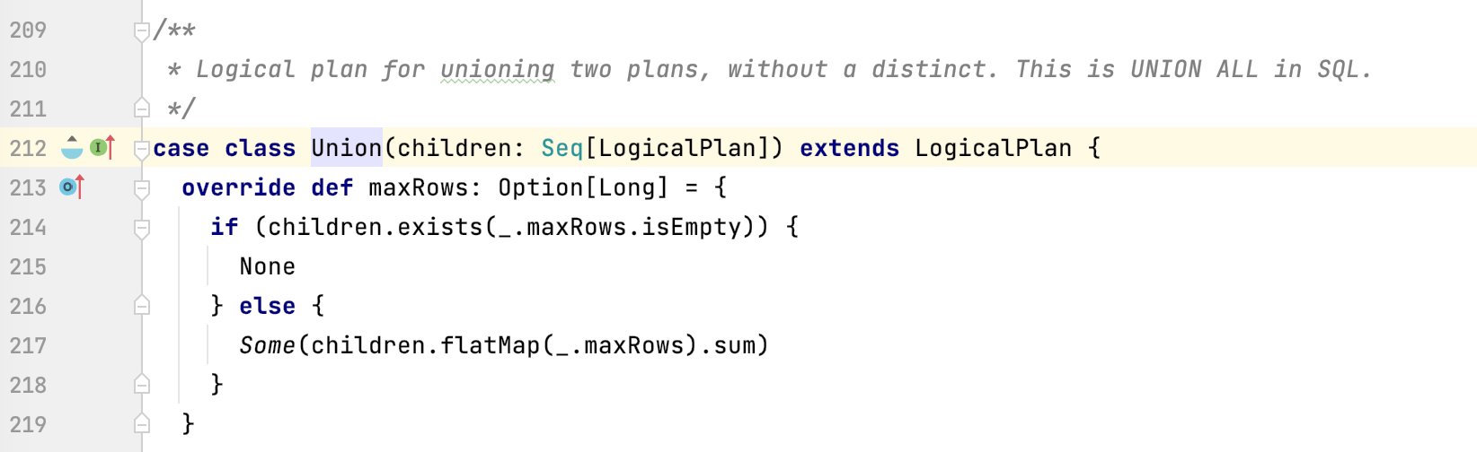
6、CombineUnions

同理CombineLimits、CombineLimits与CombineFilters类似，均是同道理的相同算子合并

 

 5.3、优化规则3：Constant folding and strength reduction 常量折叠和强度消减优化

在编译器构建中，强度消减（strength reduction）是一种编译器优化，其中昂贵的操作被等效但成本较低的操作所取代。强度降低的经典例子将循环中的“强”乘法转换为“弱”加法——这是数组寻址中经常出现的情况。强度消减的例子包括：用加法替换循环中的乘法、用乘法替换循环中的指数。
在spark中给的默认优化是：

        NullPropagation,
        ConstantPropagation,
        FoldablePropagation,
        OptimizeIn,
        ConstantFolding,
        ReorderAssociativeOperator,
        LikeSimplification,
        BooleanSimplification,
        SimplifyConditionals,
        RemoveDispensableExpressions,
        SimplifyBinaryComparison,
        PruneFilters,
        EliminateSorts,
        SimplifyCasts,
        SimplifyCaseConversionExpressions,
        RewriteCorrelatedScalarSubquery,
        EliminateSerialization,
        RemoveRedundantAliases,
        RemoveRedundantProject,
        SimplifyExtractValueOps,
        CombineConcats

1、NullPropagation 

空值替换，避免空值在SQL的语法树传播。如果没有NullPropagation，就需要在SQL语法树层面，进行层层判断是否有空值，会增加计算强度。

NullPropagation里面核心使用了scala的字面量：Literal ， 它有一个核心功能：

 

 

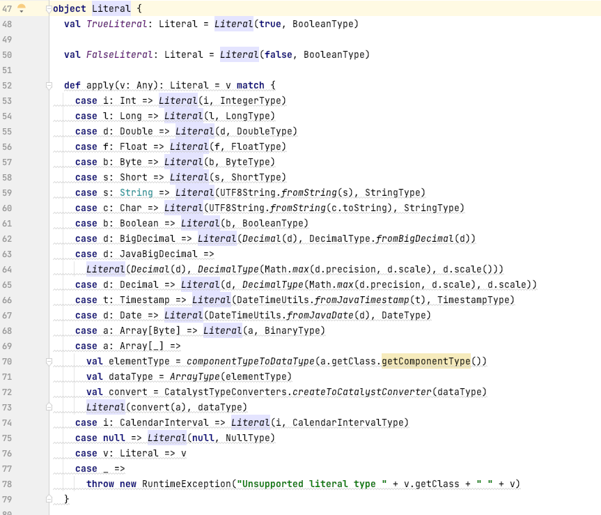
就是将系统传递的基本类型和复合类型进行转换，转成 Literal，这样在程序上就避免了null的存在

所以NullPropagation作用：

1、避免NULL值在语法树上传播，以免报错

2、减少了空值判断的次数

比如sql：

select null in (select a from table)

如果没有NullPropagation优化，其语法树为：

===========analyze===============
Filter cast(null as int) IN (list#3 [])
:  +- Project [a#0]
:     +- Project [a#0]
:        +- LocalRelation <empty>, [a#0, b#1, c#2]
+- LocalRelation <empty>, [a#0, b#1, c#2]

===========optimized===============
Filter null IN (list#3 [])
:  +- Project [a#0]
:     +- Project [a#0]
:        +- LocalRelation <empty>, [a#0, b#1, c#2]
+- LocalRelation <empty>, [a#0, b#1, c#2]

如果加上NullPropagation，其语法树为：

===========analyze===============
Filter cast(null as int) IN (list#3 [])
:  +- Project [a#0]
:     +- Project [a#0]
:        +- LocalRelation <empty>, [a#0, b#1, c#2]
+- LocalRelation <empty>, [a#0, b#1, c#2]

===========optimized===============
Filter null
+- LocalRelation <empty>, [a#0, b#1, c#2]

可以看到，经过优化之后,省去了逻辑：Filter null IN (list#3 []）

2、ConstantPropagation 常量替换

一般用于过滤条件上优化，比如有的人写sql where a = 1 and b = a+1;

这种操作如果不优化，每条数据都要计算一遍，如果数据量很大就会增加CPU计算时间

比如sql：

select a from table where a = b+1 and b = 10 and (a = c+3 or b=3) 

在没有ConstantPropagation 常量替换优化情况下，执行计划如下：

===========analyze===============
Project [a#0]
+- Filter (((a#0 = (b#1 + 1)) && (b#1 = 10)) && ((a#0 = (c#2 + 3)) || (b#1 = c#2)))
   +- Project [a#0, b#1, c#2]
      +- LocalRelation <empty>, [a#0, b#1, c#2, d#3]

===========optimized===============
Project [a#0]
+- Filter (((a#0 = (b#1 + 1)) && (b#1 = 10)) && ((a#0 = (c#2 + 3)) || (b#1 = c#2)))
   +- Project [a#0, b#1, c#2]
      +- LocalRelation <empty>, [a#0, b#1, c#2, d#3]

可以看到在Filter层，每一条数据都要做一次常量叠加的计算

使用ConstantPropagation优化后，执行计划如下：

===========analyze===============
Project [a#0]
+- Filter (((a#0 = (b#1 + 1)) && (b#1 = 10)) && ((a#0 = (c#2 + 3)) || (b#1 = c#2)))
   +- Project [a#0, b#1, c#2]
      +- LocalRelation <empty>, [a#0, b#1, c#2, d#3]

===========optimized===============
Project [a#0]
+- Filter (((a#0 = 11) && (b#1 = 10)) && ((11 = (c#2 + 3)) || (10 = c#2)))
   +- Project [a#0, b#1, c#2]
      +- LocalRelation <empty>, [a#0, b#1, c#2, d#3]

 3、FoldablePropagation 可折叠字段、属性传播（略）

 4、OptimizeIn 优化 In，空处理、重复处理

在SQL语句中in的出现频次是比较多的，必要的时候也是需要对in进行优化；

spark采用的优化in语句的方式大概遵循如下逻辑：

根据in里面是否为空，分成两种处理方式

　　1.1、如果是空，则将where a in XXX 改变成：where a

　　1.2、如果不为空，则将in里面的list集合转成Set集合来处理：val newList = ExpressionSet(list).toSeq

　　　　将list转成set后，生成newList，根据newList里面的数量分类处理如下：

　　　　1.2.1、当newList只有一个值的时候：

　　　　　　　比如where a in(1) ,则优化成where a = 1,这样就省去了遍历的操作，时间复杂度从O(n)切换成O(1)　

　　　　1.2.2、当newList的数量超过（optimizerInSetConversionThreshold默认10）的时候：

　　　　　　  spark会将in的遍历方式从list切换成Hashset，HashSet的性能是高于list的

　　　　1.2.3、当newList的数量小于原in里面的list数量：

　　　　　　 说明里面是有重读的，类似where a in ('张三' ,‘李四’，‘张三’)，因为前面已经将list转成Set方式，所以spark会做去重，让in的遍历减少

　　　　1.2.4、当newList的长度与原list的长度一致，那么处理方式不变

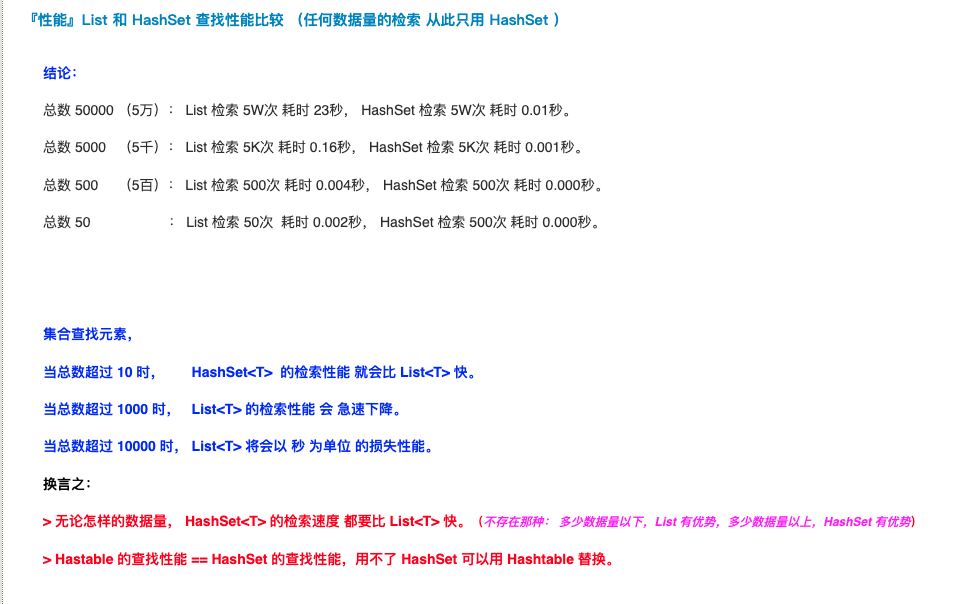
另外说明下，list和HashSet的性能对比：

 

 附上OptimizeIn源码：

object OptimizeIn extends Rule[LogicalPlan] {
  def apply(plan: LogicalPlan): LogicalPlan = plan transform {
    case q: LogicalPlan => q transformExpressionsDown {
      case In(v, list) if list.isEmpty =>
        // When v is not nullable, the following expression will be optimized
        // to FalseLiteral which is tested in OptimizeInSuite.scala
        If(IsNotNull(v), FalseLiteral, Literal(null, BooleanType))
      case expr @ In(v, list) if expr.inSetConvertible =>
        val newList = ExpressionSet(list).toSeq
        //TODO 如果 newList 长度为1， In 表达式直接转换为判断和这唯一元素是否相等的EqualTo表达式
        if (newList.length == 1
          // TODO: `EqualTo` for structural types are not working. Until SPARK-24443 is addressed,
          // TODO: we exclude them in this rule.
          && !v.isInstanceOf[CreateNamedStructLike]
          && !newList.head.isInstanceOf[CreateNamedStructLike]) {
          EqualTo(v, newList.head)
          //TODO 如果 newList  大于 spark.sql.optimizer.inSetConversionThreshold 配置的值，
          //TODO In表达式转变为 InSet 表达式，使用 hashSet 数据结构提升性能
        } else if (newList.length > SQLConf.get.optimizerInSetConversionThreshold) {
          val hSet = newList.map(e => e.eval(EmptyRow))
          InSet(v, HashSet() ++ hSet)
          /**
          如果 newList 长度小于原来的list长度相等，也就意味中有重复元素，
          这时候In 表达式转变为一个 元素更少的 In 表达式,这种情况判断方式和原来一样，也是遍历list，
          一个元素一个元素的去比较
           * */
        } else if (newList.length < list.length) {
          expr.copy(list = newList)
        } else { // newList.length == list.length && newList.length > 1
          //如果newList 长度等于原来的list长度相等，就啥也不变
          expr
        }
    }
  }
}