08-04 细分构建机器学习应用程序的流程-数据收集

目录

• 细分构建机器学习应用程序的流程-数据收集
• 一、1.1 通过sklearn生成随机数据
  • 1.1 1.1.1 make_classification()
  • 1.2 1.1.2 make_multilabel_classification()
  • 1.3 1.1.3 make_regression()
  • 1.4 1.1.4 make_blobs
  • 1.5 1.1.5 make_circles()
  • 1.6 1.1.6 make_moons
• 二、1.2 skleran自带数据集
• 三、1.3 导入UCI官网数据
• 四、1.4 导入天池比赛csv数据

人工智能从入门到放弃完整教程目录：https://www.cnblogs.com/nickchen121/p/11686958.html

细分构建机器学习应用程序的流程-数据收集

sklearn数据集官方文档地址：https://scikit-learn.org/stable/modules/classes.html#module-sklearn.datasets

sklearn数据集一览

类型	获取方式
sklearn生成的随机数据集	sklearn.datasets.make_…
sklearn自带数据集	sklearn.datasets.load_…
sklearn在线下载的数据集	sklearn.datasets.fetch_…
sklearn中加载的svmlight格式的数据集	sklearn.datasets.load_svmlight_file(…)
sklearn在mldata.org在线下载的数据集	sklearn.datasets.fetch_mldata(…)

一、1.1 通过sklearn生成随机数据

通过sklearn改变生成随机数据方法的参数，既可以获得用不尽的数据，并且数据的样本数、特征数、标记类别数、噪声数都可以自定义，非常灵活，简单介绍几个sklearn经常使用的生成随机数据的方法。

方法	用途
make_classification()	用于分类
maek_multilabel_classfication()	用于多标签分类
make_regression()	用于回归
make_blobs()	用于聚类和分类
make_circles()	用于分类
make_moons()	用于分类

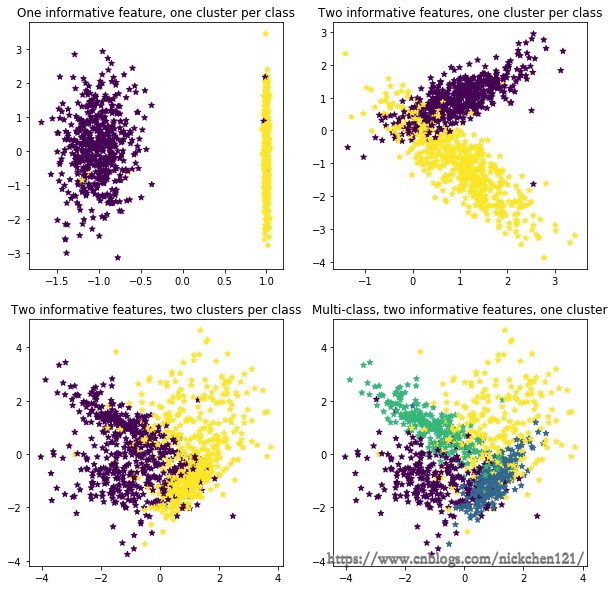
1.1 1.1.1 make_classification()

参数	解释
n_features	特征个数= n_informative（） + n_redundant + n_repeated
n_informative	多信息特征的个数
n_redundant	冗余信息，informative特征的随机线性组合
n_repeated	重复信息，随机提取n_informative和n_redundant 特征
n_classes	分类类别
n_clusters_per_class	某一个类别是由几个cluster构成的

import numpy as np
import pandas as pd
import matplotlib.pyplot as plt
from matplotlib.font_manager import FontProperties
from sklearn import datasets
%matplotlib inline
font = FontProperties(fname='/Library/Fonts/Heiti.ttc')

from sklearn import datasets
try:
    X1, y1 = datasets.make_classification(
        n_samples=50, n_classes=3, n_clusters_per_class=2, n_informative=2)
    print(X1.shape)
except Exception as e:
    print('error:{}'.format(e))

# 下面错误信息n_classes * n_clusters_per_class must be smaller or equal 2 ** n_informative，
# 当n_clusters_per_class=2时，意味着该生成随机数的n_classes应该小于2，可以理解成一分类或二分类

error:n_classes * n_clusters_per_class must be smaller or equal 2 ** n_informative

import matplotlib.pyplot as plt
%matplotlib inline

plt.figure(figsize=(10, 10))

plt.subplot(221)
plt.title("One informative feature, one cluster per class", fontsize=12)
X1, y1 = datasets.make_classification(n_samples=1000, random_state=1, n_features=2, n_redundant=0, n_informative=1,
                                      n_clusters_per_class=1)
plt.scatter(X1[:, 0], X1[:, 1], marker='*', c=y1)

plt.subplot(222)
plt.title("Two informative features, one cluster per class", fontsize=12)
X1, y1 = datasets.make_classification(n_samples=1000, random_state=1, n_features=2, n_redundant=0, n_informative=2,
                                      n_clusters_per_class=1)
plt.scatter(X1[:, 0], X1[:, 1], marker='*', c=y1)

plt.subplot(223)
plt.title("Two informative features, two clusters per class", fontsize=12)
X1, y1 = datasets.make_classification(
    n_samples=1000, random_state=1, n_features=2, n_redundant=0, n_informative=2)
plt.scatter(X1[:, 0], X1[:, 1], marker='*', c=y1)


plt.subplot(224)
plt.title("Multi-class, two informative features, one cluster",
          fontsize=12)
X1, y1 = datasets.make_classification(n_samples=1000, random_state=1, n_features=2, n_redundant=0, n_informative=2,
                                      n_clusters_per_class=1, n_classes=4)
plt.scatter(X1[:, 0], X1[:, 1], marker='*', c=y1)
plt.show()

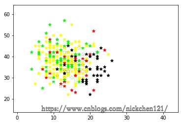
1.2 1.1.2 make_multilabel_classification()

X1, y1 = datasets.make_multilabel_classification(
    n_samples=1000, n_classes=4, n_features=2, random_state=1)
datasets.make_multilabel_classification()

print('样本维度:{}'.format(X1.shape))

# 一个样本可能有多个标记
print(y1[0:5, :])

样本维度:(1000, 2)
[[1 1 0 0]
 [0 0 0 0]
 [1 1 0 0]
 [0 0 0 1]
 [0 0 0 0]]

plt.scatter(X1[:, 0], X1[:, 1], marker='*', c=y1)
plt.show()

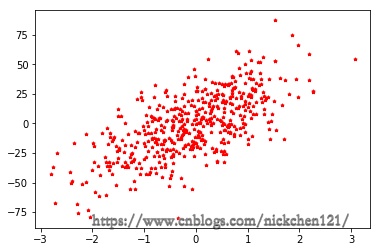
1.3 1.1.3 make_regression()

import matplotlib.pyplot as plt
%matplotlib inline
from sklearn import datasets
X1, y1 = datasets.make_regression(n_samples=500, n_features=1, noise=20)
plt.scatter(X1, y1, color='r', s=10, marker='*')
plt.show()

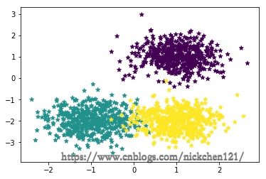
1.4 1.1.4 make_blobs

# 生成3个簇的中心点
centers = [[1, 1], [-1, -2], [1, -2]]

X1, y1 = datasets.make_blobs(
    n_samples=1500, centers=centers, n_features=2, random_state=1, shuffle=False, cluster_std=0.5)

print('样本维度:{}'.format(X1.shape))

# plt.scatter(X1[0:500, 0], X1[0:500, 1], s=10, label='cluster1')
# plt.scatter(X1[500:1000, 0], X1[500:1000, 1], s=10, label='cluster2')
# plt.scatter(X1[1000:1500, 0], X1[1000:1500, 1], s=10, label='cluster3')
plt.scatter(X1[:, 0], X1[:, 1], marker='*', c=y1)
plt.show()

样本维度:(1500, 2)

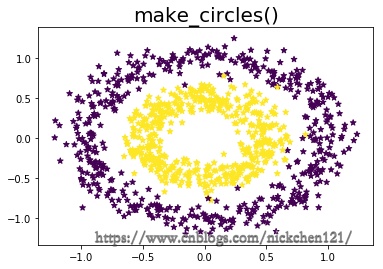
1.5 1.1.5 make_circles()

X1, y1 = datasets.make_circles(
    n_samples=1000, random_state=1, factor=0.5, noise=0.1)

print('样本维度:{}'.format(X1.shape))

plt.scatter(X1[:, 0], X1[:, 1], marker='*', c=y1)
plt.title('make_circles()', fontsize=20)
plt.show()

样本维度:(1000, 2)

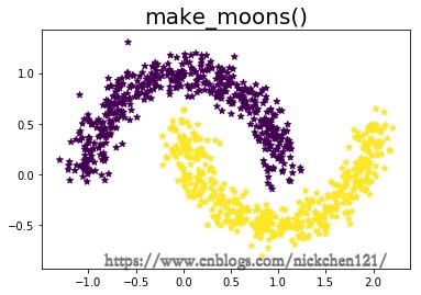
1.6 1.1.6 make_moons

X1, y1 = datasets.make_moons(n_samples=1000, noise=0.1, random_state=1)

print('样本维度:{}'.format(X1.shape))

plt.scatter(X1[:, 0], X1[:, 1], marker='*', c=y1)
plt.title('make_moons()', fontsize=20)
plt.show()

样本维度:(1000, 2)

二、1.2 skleran自带数据集

方法	描述	用途
load_iris()	鸢尾花数据集	用于分类或聚类
load_digits()	手写数字数据集	用于分类
load_breast_cancer()	乳腺癌数据集	用于分类
load_boston()	波士顿房价数据集	用于回归
load_linnerud()	体能训练数据集	用于回归
load_sample_image(name)	图像数据集

# 鸢尾花数据集
iris = datasets.load_iris()
iris['target_names']

array(['setosa', 'versicolor', 'virginica'], dtype='<U10')

# 手写数字数据集
digits = datasets.load_digits()
digits['target_names']

array([0, 1, 2, 3, 4, 5, 6, 7, 8, 9])

# 乳腺癌数据集
breast = datasets.load_breast_cancer()
breast['target_names']

array(['malignant', 'benign'], dtype='<U9')

# 波士顿房价数据集
boston = datasets.load_boston()
boston['feature_names']

array(['CRIM', 'ZN', 'INDUS', 'CHAS', 'NOX', 'RM', 'AGE', 'DIS', 'RAD',
       'TAX', 'PTRATIO', 'B', 'LSTAT'], dtype='<U7')

# 体能训练数据集
linnerud = datasets.load_linnerud()
linnerud['feature_names']

['Chins', 'Situps', 'Jumps']

# 图像数据集
china = datasets.load_sample_image('china.jpg')
plt.axis('off')
plt.title('中国颐和园图像', fontproperties=font, fontsize=20)
plt.imshow(china)
plt.show()

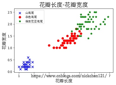
三、1.3 导入UCI官网数据

UCI官网：http://archive.ics.uci.edu/ml/datasets.html

df = pd.read_csv(
    'http://archive.ics.uci.edu/ml/machine-learning-databases/iris/iris.data', header=None)

# 取出前100行的第五列即生成标记向量
y = df.iloc[0:100, 4].values
# 如果标记为'Iris-versicolor'则赋值1，否则赋值-1
y = np.where(y == 'Iris-versicolor', 1, -1)

# 取出前100行的第一列和第三列的特征即生成特征向量
X = df.iloc[:, [2, 3]].values

plt.scatter(X[:50, 0], X[:50, 1], color='b', s=50, marker='x', label='山鸢尾')
plt.scatter(X[50:100, 0], X[50:100, 1], color='r',
            s=50, marker='o', label='杂色鸢尾')
plt.scatter(X[100:150, 0], X[100:150, 1], color='g',
            s=50, marker='*', label='维吉尼亚鸢尾')
plt.xlabel('花瓣长度', fontproperties=font, fontsize=15)
plt.ylabel('花瓣宽度', fontproperties=font, fontsize=15)
plt.title('花瓣长度-花瓣宽度', fontproperties=font, fontsize=20)
plt.legend(prop=font)
plt.show()

四、1.4 导入天池比赛csv数据

本次以天池比赛中的葡萄酒质量研究的数据为例，下载地址：https://tianchi.aliyun.com/dataset/dataDetail?dataId=44

上图可以看出，葡萄酒质量的数据是存放在.csv文件当中，我们首先把csv文件下载到本地，然后可以使用pandas做处理。

# csv可以看成普通文本文件，pandas可以使用read_csv读取
df = pd.read_csv('winequality-red.csv')
df[:2]

	fixed acidity;"volatile acidity";"citric acid";"residual sugar";"chlorides";"free sulfur dioxide";"total sulfur dioxide";"density";"pH";"sulphates";"alcohol";"quality"
7.4;0.7;0;1.9;0.076;11;34;0.9978;3.51;0.56;9.4;5
7.8;0.88;0;2.6;0.098;25;67;0.9968;3.2;0.68;9.8;5

# sep参数相当于规定csv文件数据的分隔符
df = pd.read_csv('winequality-red.csv', sep=';')
df[:2]

	fixed acidity	volatile acidity	citric acid	residual sugar	chlorides	free sulfur dioxide	total sulfur dioxide	density	pH	sulphates	alcohol	quality
7.4	0.70	0.0	1.9	0.076	11.0	34.0	0.9978	3.51	0.56	9.4	5
7.8	0.88	0.0	2.6	0.098	25.0	67.0	0.9968	3.20	0.68	9.8	5

# 获取特征值
X = df.iloc[:2, :-1].values
X

array([[ 7.4   ,  0.7   ,  0.    ,  1.9   ,  0.076 , 11.    , 34.    ,
         0.9978,  3.51  ,  0.56  ,  9.4   ],
       [ 7.8   ,  0.88  ,  0.    ,  2.6   ,  0.098 , 25.    , 67.    ,
         0.9968,  3.2   ,  0.68  ,  9.8   ]])

# 获取标记值
y = df.iloc[:2, -1].values
y

array([5, 5])