

import pandas as pd
import numpy as np
%matplotlib inline
df=pd.DataFrame({'A':['foo','bar','foo','bar','foo','bar','foo','foo'],
                 'B':['one','one','two','three','two','one','one','three'],
                'C':np.random.randn(8),
                'D':np.random.randn(8)})
| A | B | C | D | |
|---|---|---|---|---|
| 0 | foo | one | 1.204416 | -0.132263 |
| 1 | bar | one | -0.395242 | 0.843990 |
| 2 | foo | two | 0.471486 | -0.320840 |
| 3 | bar | three | 0.888173 | 0.308669 |
| 4 | foo | two | 0.368766 | -1.033001 |
| 5 | bar | one | 0.269763 | 0.562003 |
| 6 | foo | one | -1.073367 | -0.999027 |
| 7 | foo | three | -0.140331 | 1.021435 |
一、使用分组聚合函数做统计
1、单列groupby,查询所有数据列的统计
df.groupby('A').sum()
Out[9]:
1)A列变成索引
2)因为B列不是数值,被忽略了
2、多个列的groupby,查询所有数据列的统计
2.1、二维索引
df.groupby(['A','B']).mean()
| C | D | ||
|---|---|---|---|
| A | B | ||
| bar | one | -0.062739 | 0.702996 |
| three | 0.888173 | 0.308669 | |
| foo | one | 0.065524 | -0.565645 |
| three | -0.140331 | 1.021435 | |
| two | 0.420126 | -0.676920 |
2.2、取消索引,注意看区别
df.groupby(['A','B'],as_index=False).mean()
| A | B | C | D | |
|---|---|---|---|---|
| 0 | bar | one | 1.190061 | -0.965350 |
| 1 | bar | three | -0.748586 | 0.305491 |
| 2 | foo | one | -0.294912 | 0.369032 |
| 3 | foo | three | -2.015986 | -1.375908 |
| 4 | foo | two | 1.334180 | -0.175115 |
3、同时查看多种数据统计
3.1查看所有列的多种统计
#同时查看多种数据统计
df.groupby('B').agg([np.sum,np.mean,np.std])
3.2查看选定列的多种统计
df.groupby('A')['C'].agg([np.sum,np.mean,np.std])


#或者可以写成
df.groupby('A').agg([np.sum,np.mean,np.std])['C']
3.3不同的列用不同的统计方法:传入一个字典
df.groupby('A').agg({'C':np.mean,'D':np.sum})
二、用for遍历groupby
2.1
#用for循环遍历
c=df.groupby('A')
for name,group in c:
    print(name)
    print(group)
bar
     A      B         C         D         从输出结果看出,name就是A列的取值,group就是按A列不同取值的分组结果
1 bar one 0.468276 -0.288917
3 bar three 0.322501 -0.115328
5 bar one 0.288724 0.442796
foo
A B C D
0 foo one 0.684513 1.131908
2 foo two -1.045012 -0.623831
4 foo two -1.415123 0.413129
6 foo one -0.581241 0.014809
7 foo three -0.421476 -1.613835
2.2获取单个分组的数据
c.get_group('bar')
| A | B | C | D | |
|---|---|---|---|---|
| 1 | bar | one | 0.468276 | -0.288917 |
| 3 | bar | three | 0.322501 | -0.115328 |
| 5 | bar | one | 0.288724 | 0.442796 |
2.3遍历多个列聚合的分组
d=df.groupby(['A','B'])
for name,group in d:
    print(name)
    print(group)
('bar', 'one')
     A    B         C         D          从输出结果可以看出,name就是A、B列中的二元元组
1  bar  one  0.470414 -0.511101
5  bar  one  1.048932 -0.670548
('bar', 'three')
     A      B         C         D
3  bar  three -0.094712 -0.528441
('foo', 'one')
     A    B         C         D
0  foo  one -1.004307 -0.651963
6  foo  one -1.411104  0.773112
('foo', 'three')
     A      B         C         D
7  foo  three  0.539208  0.680722
('foo', 'two')
     A    B         C         D
2  foo  two -1.396579  1.218200
4  foo  two -0.950124 -1.447044
也可以把元组传入get_groupby
d.get_group(('foo','one'))
| A | B | C | D | |
|---|---|---|---|---|
| 0 | foo | one | -1.004307 | -0.651963 |
| 6 | foo | one | -1.411104 | 0.773112 |
2.4 可以直接查询group的某几列,生成series或dataframe
d=df.groupby(['A','B'])
for name,group in d["C"]:
    print(name)
    print(group)
('bar', 'one')
1   -0.294708
5   -0.907187
Name: C, dtype: float64
('bar', 'three')
3   -1.266895
Name: C, dtype: float64
('foo', 'one')
0    0.583220
6    0.704326
Name: C, dtype: float64
('foo', 'three')
7   -0.963204
Name: C, dtype: float64
('foo', 'two')
2   -0.150334
4    1.051601
Name: C, dtype: float64
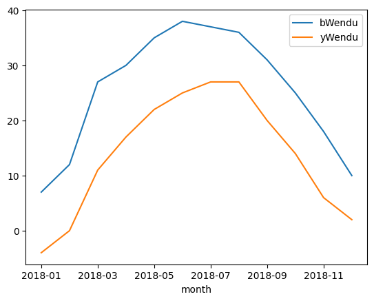
三、实例:对北京2018年天气表进行按月统计
#读取文件
fpath='./beijing_tianqi/beijing_tianqi_2018.csv'
df=pd.read_csv(fpath)
#将气温格式化为数字
df.loc[:,'bWendu']=df['bWendu'].str.replace('℃','').astype('int32')
df.loc[:,'yWendu']=df['yWendu'].str.replace('℃','').astype('int32')
#表格添加一列“月份”
df['month']=df['ymd'].str[:7]
#求每个月的最低温和最高温的最大值
ata=df.groupby('month')['bWendu','yWendu'].max()
data.plot()

#求每个月最高温的最大、最低温的最小、控制质量的平均
grop_data=df.groupby('month').agg({'bWendu':np.max,'yWendu':np.min,'aqi':np.mean})
| bWendu | yWendu | aqi | |
|---|---|---|---|
| month | |||
| 2018-01 | 7 | -12 | 60.677419 |
| 2018-02 | 12 | -10 | 78.857143 |
| 2018-03 | 27 | -4 | 130.322581 |
| 2018-04 | 30 | 1 | 102.866667 |
| 2018-05 | 35 | 10 | 99.064516 |
| 2018-06 | 38 | 17 | 82.300000 |
| 2018-07 | 37 | 22 | 72.677419 |
| 2018-08 | 36 | 20 | 59.516129 |
| 2018-09 | 31 | 11 | 50.433333 |
| 2018-10 | 25 | 1 | 67.096774 |
| 2018-11 | 18 | -4 | 105.100000 |
| 2018-12 | 10 | -12 | 77.354839 |
1  bar    one  0.468276 -0.288917
3  bar  three  0.322501 -0.115328
5  bar    one  0.288724  0.442796
foo
     A      B         C         D
0  foo    one  0.684513  1.131908
2  foo    two -1.045012 -0.623831
4  foo    two -1.415123  0.413129
6  foo    one -0.581241  0.014809
7  foo  three -0.421476 -1.613835
