TensorFlow2.1入门学习笔记(7)——损失函数
TensorFlow2.0入门学习笔记(7)——损失函数
损失函数(loss):
预测值(y)与已知答案(y_)的差距
神经网络的优化目标:loss最小 \(\Rightarrow \left\{\begin{array}{lr}mse(Mean Aquared Error) \\自定义 \\ce(Cross Entropy)\end{array}\right.\)
均方误差mse:loss_mse = tf.reduce_mean(tf.square(y_-y))
\[MSE(y\_,y)=\frac{\sum_{i=1}^{n}(y-y\_)^2}{n}
\]
- 例
预测酸奶日销量y,x1、x2是影响日销量的因素。
建模前,应预先采集的数据有:每日x1、x2和销量y_(即已知答案,最佳的情况:产量=销量)
拟造数据集X,Y:y_=x1+x2
噪声:-0.05~+0.05
拟合可以预算销量的函数
import tensorflow as tf
import numpy as np
SEED = 23455
rdm = np.random.RandomState(seed=SEED) # 生成[0,1)之间的随机数
x = rdm.rand(32, 2)
y_ = [[x1 + x2 + (rdm.rand() / 10.0 - 0.05)] for (x1, x2) in x] # 生成噪声[0,1)/10=[0,0.1); [0,0.1)-0.05=[-0.05,0.05)
x = tf.cast(x, dtype=tf.float32)
w1 = tf.Variable(tf.random.normal([2, 1], stddev=1, seed=1))
epoch = 15000
lr = 0.002
for epoch in range(epoch):
with tf.GradientTape() as tape:
y = tf.matmul(x, w1)
loss_mse = tf.reduce_mean(tf.square(y_ - y))
grads = tape.gradient(loss_mse, w1)
w1.assign_sub(lr * grads)
if epoch % 500 == 0:
print("After %d training steps,w1 is " % (epoch))
print(w1.numpy(), "\n")
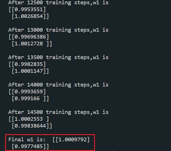
print("Final w1 is: ", w1.numpy())
- 运行结果
自定义损失函数:
如预测产品销量,预测多了,损失成本;预测少了,损失利润。若利润\(\neq\)成本,则mse产生的loss无法利益最大化。
自定义损失函数:\(loss(y\_,y)=\sum_{n}f(y\_,y)\)
\[f(y\_,y)=\left\{\begin{array}{lr}PROFIT*(y\_-y)&y<y\_ \\COST*(y\_-y)&y\geq y\_\end{array}\right.
\]
loss_zdy=tf.reduce_sum(tf.where(tf.greater(y,y_),COST(y-y_),PROFIT(y_-y)))
如:预测酸奶销量,酸奶成本(COST)1元,酸奶利润(PROFIT)99元
预测少了损失利润99元,预测多了损失1元,希望生成的预测函数往多了预测
import tensorflow as tf
import numpy as np
SEED = 23455
COST = 1
PROFIT = 99
rdm = np.random.RandomState(SEED)
x = rdm.rand(32, 2)
y_ = [[x1 + x2 + (rdm.rand() / 10.0 - 0.05)] for (x1, x2) in x] # 生成噪声[0,1)/10=[0,0.1); [0,0.1)-0.05=[-0.05,0.05)
x = tf.cast(x, dtype=tf.float32)
w1 = tf.Variable(tf.random.normal([2, 1], stddev=1, seed=1))
epoch = 10000
lr = 0.002
for epoch in range(epoch):
with tf.GradientTape() as tape:
y = tf.matmul(x, w1)
loss = tf.reduce_sum(tf.where(tf.greater(y, y_), (y - y_) * COST, (y_ - y) * PROFIT))
grads = tape.gradient(loss, w1)
w1.assign_sub(lr * grads)
if epoch % 500 == 0:
print("After %d training steps,w1 is " % (epoch))
print(w1.numpy(), "\n")
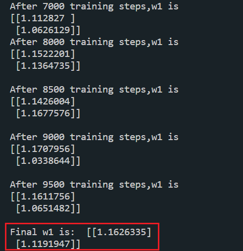
print("Final w1 is: ", w1.numpy())
- 运行结果
交叉熵损失函数:tf.losses.categorical_crossentropy(y_,y)
\[H(y\_,y)=-\sum y\_*lny
\]
CE(Cross Entropy):表示两个概率分布之间的距离
eg.二分类 已知答案y_=(1,0)
预测\(y_1\)=(0.6,0.4) \(y_2\)=(0.8,0.2)哪个更接近标准答案
\(H_1\)((1,0),(0.6,0.4))=-(1\(*\)ln0.6 + 0\(*\)ln0.4)\(\approx\)-(-0.511 + 0) = 0.511
\(H_2\)((1,0),(0.8,0.2))=-(1\(*\)ln0.8 + 0\(*\)ln0.2)\(\approx\)-(-0.223 + 0) = 0.223
因为\(H_1>H_2\),所以\(y_2\)预测更准确
import tensorflow as tf
loss_ce1 = tf.losses.categorical_crossentropy([1, 0], [0.6, 0.4])
loss_ce2 = tf.losses.categorical_crossentropy([1, 0], [0.8, 0.2])
print("loss_ce1:", loss_ce1)
print("loss_ce2:", loss_ce2)
- 运行结果

softmax与交叉熵解和:tf.nn.softmax_cross_entropy_with_logits(y_,y)
输出先过softmax函数,再计算y与y_的交叉熵损失函数
# softmax与交叉熵损失函数的结合
import tensorflow as tf
import numpy as np
y_ = np.array([[1, 0, 0], [0, 1, 0], [0, 0, 1], [1, 0, 0], [0, 1, 0]])
y = np.array([[12, 3, 2], [3, 10, 1], [1, 2, 5], [4, 6.5, 1.2], [3, 6, 1]])
y_pro = tf.nn.softmax(y)
loss_ce1 = tf.losses.categorical_crossentropy(y_,y_pro)
loss_ce2 = tf.nn.softmax_cross_entropy_with_logits(y_, y)
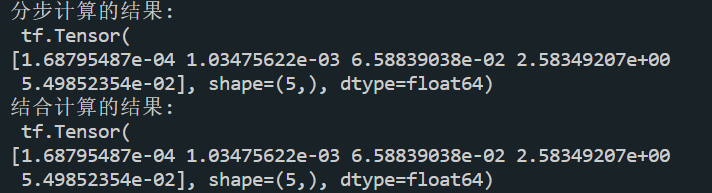
print('分步计算的结果:\n', loss_ce1)
print('结合计算的结果:\n', loss_ce2)
- 运行结果:
主要学习的资料,西安科技大学:神经网络与深度学习——TensorFlow2.0实战,北京大学:人工智能实践Tensorflow笔记

 浙公网安备 33010602011771号