08_线性回归详解

线性回归详解

1、包导入与数据创建

import numpy as np
import matplotlib
import matplotlib.pyplot as plt

# 绘图全局参数设置
config = {
    "font.family": 'Times New Roman',
    "font.size": 14,
    "font.serif": 'Simsun',
}
matplotlib.rcParams.update(config)

导入需要的数据处理包numpy和绘图包matplotlib

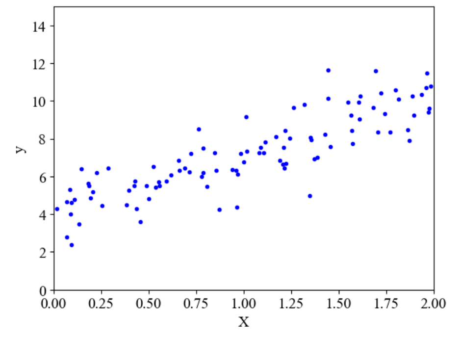
# 随机生成100个样本

X = 2 * np.random.rand(100, 1)
# 使用一次线性公式4+3*x并增加随机数来模拟噪音影响
y = 4 + 3 * X + np.random.randn(100, 1)

# 显示生成的数据
plt.plot(X, y, 'b.')
plt.xlabel('X')
plt.ylabel('y')
plt.axis([0, 2, 0, 15])
plt.show()

2、直接求解法

损失函数：

\(\displaystyle J(\theta) = \frac12\sum^m_{i=1}(y^i - \theta^Tx^i)^2=\frac12\sum^m_{i=1}(h_\theta(x^i)-y^i)^2 = \frac12(X\theta - y)^T(X\theta-y)\)

损失函数求导：

\(\displaystyle \nabla_\theta J(\theta)=\nabla_\theta [\frac12(X\theta - y)^T(X\theta-y)]=\nabla_\theta[\frac12(\theta^TX^T-y^T)(X\theta-y)]\)

\(\displaystyle =\nabla_\theta[\frac12(\theta^TX^TX\theta-\theta^TX^Ty-y^TX\theta+y^Ty)]\)

\(\displaystyle =\frac12(2X^TX\theta-X^Ty-(y^TX)^T)=X^TX\theta-X^Ty\)

让损失函数求导后等于0建立方程求得：

\(\displaystyle \theta = (X^TX)^{-1}X^Ty\)

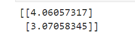
直接求解

# 增加一列 1, 作为偏置项参数
X_b = np.c_[np.ones((100, 1)), X]
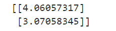
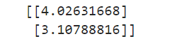
theta_best = np.linalg.inv(X_b.T.dot(X_b)).dot(X_b.T).dot(y)
print(theta_best)

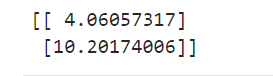
# 预测
X_new = np.array([[0], [2]])
X_new_b = np.c_[np.ones((2, 1)), X_new]
y_predict = X_new_b.dot(theta_best)
print(y_predict)

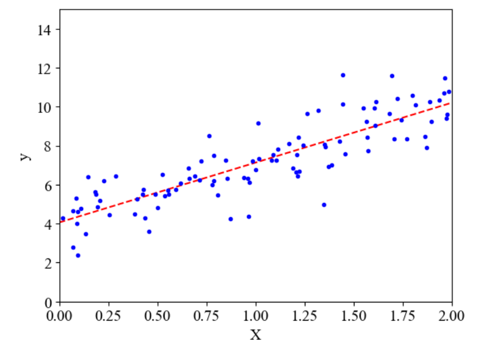
# 绘制回归线
plt.plot(X_new, y_predict, 'r--')
plt.plot(X, y, 'b.')
plt.xlabel('X')
plt.ylabel('y')
plt.axis([0, 2, 0, 15])
plt.show()

from sklearn.linear_model import LinearRegression

# 这里使用的是直接求导的方程方法
lin_reg = LinearRegression()
lin_reg.fit(X, y)
print(lin_reg.coef_)
print(lin_reg.intercept_)

• 优点：得到的结果是最优解
• 缺点：由于求解公式中有求逆的存在，而并不是所有的矩阵都能求逆，并且在数据量比较大时，计算速度比较慢，所以有了梯度下降的方法

3、梯度下降准备

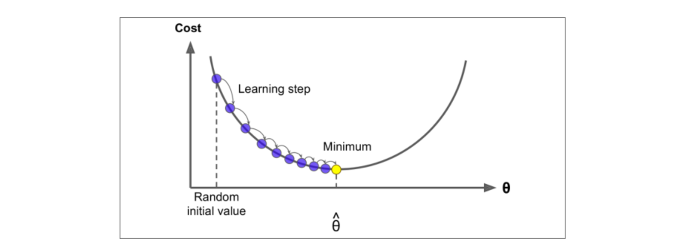
• 正常梯度下降：先随机选取一个初始点，然后一步步逼近最优解

  

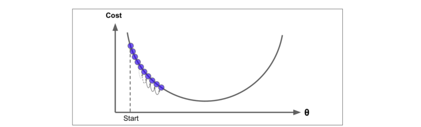
• 步长太小：会导致求解时间长

  

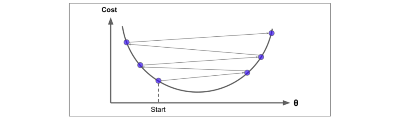
• 步长太大：求解过程跌宕起伏，得到的解不好，所以一般步长宁可小也不能大

  

• 局部最优解：在线性回归中一般都不会有局部最优解，因为线性回归是凸函数，但是在有些问题中会存在这样的问题

  

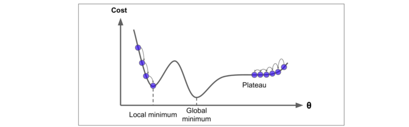
  对于这种问题需要多做几组实验，在不同的位置选取初始点，在绝大部分机器学习问题中都不存在局部最优解

• 数据处理标准化：让所有特征数据的取值范围一致，从而方便求解，拿到数据之后基本上都需要进行标准化操作

  

  标准化只是数据预处理中的一种，在sklearn中有一个专门的预处理模块 sklearn.preprocessing，里面有很多预处理的函数

4、批量梯度下降

公式：

\(\displaystyle J(\theta) = \frac1{2m}\sum^m_{i=1}(h_\theta(x^i)-y^i)^2\)

\(\displaystyle \frac{\partial J(\theta)}{\partial \theta_j} = \frac1m \sum^m_{i=1}(h_\theta(x^i)-y^i)x^i_j\)

\(\displaystyle \theta_j' = \theta_j - \alpha\frac1m \sum^m_{i=1}(h_\theta(x^i)-y^i)x^i_j\)

\(\displaystyle \theta' = \theta - \alpha \frac1m X^T(X\theta - y)\)

# 批量梯度下降
eta = 0.2
n_iterations = 1000
m = len(X_b)
theta = np.random.randn(2, 1)
for iteration in range(n_iterations):
    gradients = 1/m*X_b.T.dot(X_b.dot(theta) - y)
    theta = theta - eta * gradients
print(theta)

我们来尝试不同学习率对模型的影响

# 绘图
theta_path_bgd = []
def plot_gradient_descent(theta, eta, theta_path = None):
    m = len(X_b)
    plt.plot(X, y, 'b.')
    n_iterations = 1000
    for iteration in range(n_iterations):
        y_predict = X_new_b.dot(theta)
        gradients = 1/m*X_b.T.dot(X_b.dot(theta) - y)
        theta = theta - eta * gradients
        if theta_path:
            theta_path.append(theta)
        
        plt.plot(X_new, y_predict, 'r-')
        plt.xlabel('X_1')
        plt.axis([0, 2, 0, 15])
        plt.title(f'eta = {eta}')

theta = np.random.randn(2, 1)

plt.figure(figsize=(10, 4))
plt.subplot(131)
plot_gradient_descent(theta, eta = 0.02)
plt.subplot(132)
plot_gradient_descent(theta, eta = 0.2)
plt.subplot(133)
plot_gradient_descent(theta, eta = 1)

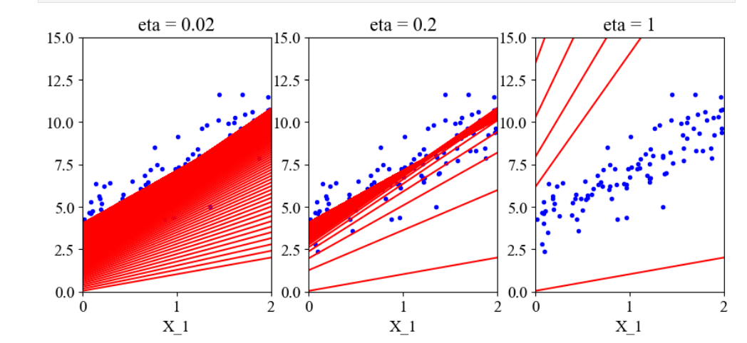
可以直观的看到，当学习率太小时，模型需要很多步才能达到最优解；而学习率太大时，模型确不能达到最优解。所以在实际运用中，学习率宁可小也不能大

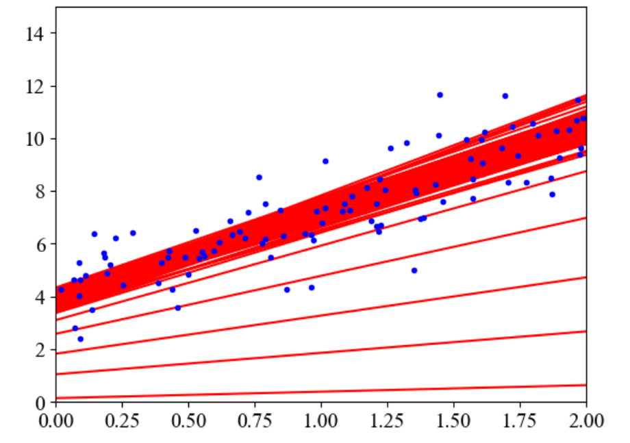
5、随机梯度下降

公式：

\(\displaystyle \theta' = \theta - \alpha(h_\theta(x^i)-y^i)x^i_j = \theta - \alpha(x_j^i\theta-y^i)x^i_j\)

theta_path_sgd = []
m = len(X_b)
n_epochs = 10

t0 = 5
t1 = 50
theta = np.random.randn(2, 1)

def learning_schedule(t):
    return t0 / (t1 + t)

for epoch in range(n_epochs):
    for i in range(m):
        if epoch < 4 and i % 2 == 0:
            y_predict = X_new_b.dot(theta)
            plt.plot(X_new, y_predict, 'r-')
        random_index = np.random.randint(m)
        xi = X_b[random_index:random_index+1]
        yi = y[random_index:random_index+1]
        gradients = xi.T.dot(xi.dot(theta) - yi)
        eta = learning_schedule(epoch * m + 1)
        theta = theta - eta*gradients
        theta_path_sgd.append(theta)
        
plt.plot(X, y, 'b.')
plt.axis([0, 2, 0, 15])
plt.show()

6、小批量随机梯度下降

公式：

\(\displaystyle \theta_j' = \theta_j - \alpha\frac1{batch} \sum^{i+batch-1}_{k=1}(h_\theta(x^k)-y^k)x^k_j\)

\(\displaystyle = \theta_j - \alpha \frac1{batch} X_j^T(X_j\theta - y_j)\)

theta_path_mgd = []
n_epochs = 10
minibatch = 16
theta = np.random.randn(2, 1)

for t, epoch in enumerate(range(n_epochs)):
    shuffled_indices = np.random.permutation(m)
    X_b_shuffled = X_b[shuffled_indices]
    y_shuffled = y[shuffled_indices]
    for i in range(0, m, minibatch):
        xi = X_b_shuffled[i:i+minibatch]
        yi = y_shuffled[i:i+minibatch]
        gradients = 1 / minibatch * xi.T.dot(xi.dot(theta) - yi)
        eta = learning_schedule(t)
        theta = theta - eta * gradients
        theta_path_mgd.append(theta)
print(theta)

7、三种梯度下降对比

theta_path_bgd = np.array(theta_path_bgd)
theta_path_sgd = np.array(theta_path_sgd)
theta_path_mgd = np.array(theta_path_mgd)

plt.figure(figsize=(8, 4))
plt.plot(theta_path_sgd[:, 0], theta_path_sgd[:, 1], 'g-+', markersize=3, linewidth=1, label='SGD')
plt.plot(theta_path_mgd[:, 0], theta_path_mgd[:, 1], 'b-o', markersize=3, linewidth=1, label='MGD')
plt.plot(theta_path_bgd[:, 0], theta_path_bgd[:, 1], 'r-s', markersize=3, linewidth=1, label='BGD')
plt.legend(loc='upper right')
plt.axis([3, 4.2, 2.5, 4.5])
plt.show()

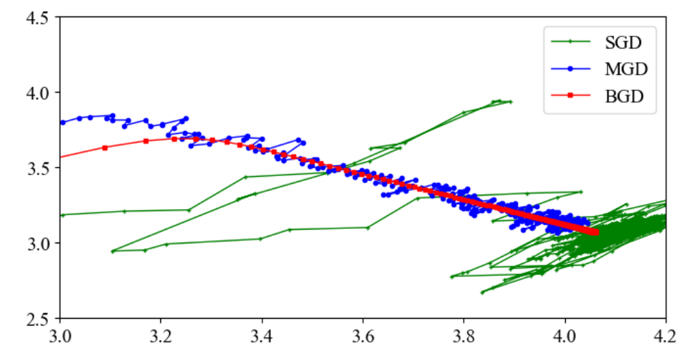
看红色的线，可以看到批量梯度下降像是直接往最终结果的方向走；再看蓝色的线，小批量随机梯度下降也是往最终结果方向前进，但是过程有一些波动；最后看绿色的线，随机梯度下降的前进方向波动更大。