
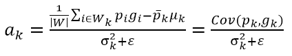
由上篇导向滤波算法分析,根据(5)~(8)式就可以计算输出图像Q
 (5)
(5)
![]() (6)
(6)
![]() (7)
(7)
![]() (8)
(8)
其中![]() ,
,![]() ,/ai和/bi的结果要计算所有覆盖了像素i的窗口Wk的ak和bk的平均值。除了用平均值,在实际应用中,我还看到过其他的计算/ai和/bi的方法。比如根据像素i在窗口Wk的位置,给予不同的权重。如果i距离窗口Wk的中心位置越远,则给予ak和bk越低的权重。如果i位于窗口中心,则ak和bk有最高的权重。最常用的就是用高斯分布来给予不同的权重。这样考虑到了附近像素距离远近对i影响的大小,最后的结果会更精确一些。
,/ai和/bi的结果要计算所有覆盖了像素i的窗口Wk的ak和bk的平均值。除了用平均值,在实际应用中,我还看到过其他的计算/ai和/bi的方法。比如根据像素i在窗口Wk的位置,给予不同的权重。如果i距离窗口Wk的中心位置越远,则给予ak和bk越低的权重。如果i位于窗口中心,则ak和bk有最高的权重。最常用的就是用高斯分布来给予不同的权重。这样考虑到了附近像素距离远近对i影响的大小,最后的结果会更精确一些。
这里我还是用最简单的平均值的方法来计算/ai和/bi。我们前面已经假定了在窗口Wk内,ak和bk是常数,因此ak和bk只和Wk的位置有关。取Wk为半径为r的方形窗口,使窗口的中心像素位置遍历整个图像,那么就使Wk取到了不同的所有位置,在每个位置计算出相应的ak和bk。所有的ak和bk组成了和输入图像P相同长宽维度的数据集合,记为A和B。对于任意像素i,/ai和/bi即分别为以i为中心半径r的窗口Wk内A和B的数据均值,这不正是我们熟悉的图像均值模糊的算法吗?而图像均值模糊有几种比较成熟的快速算法,比如积分图算法和基于直方图的快速算法。只要有了A和B,就可以方便的应用均值模糊得出/ai和/bi,从而应用(8)计算出输出图像Q。
为了计算A和B,从(6)式看到,需要分别计算输入图像P和导向图G的均值模糊结果。而(5)式需要计算导向图G的方差,还有P和G的协方差。方差和协方差都涉及到乘积的求和计算,可以由下面的公式,通过积分图来计算。这两个公式很容易推导出来,就不赘述了。
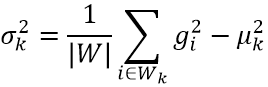
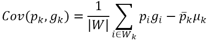
一个平方和,一个乘积和都可以用积分图来计算。只是要注意当图像足够大的时候,要用合适的数据类型。假设像素的数据范围是0~255的整型,如果平方积分图用32位的整型数据,那么只能支持最大256x256大小的图像。超过这个大小,就必须要用64位的整型了。下面给出使用模板函数的乘积积分图函数,可以根据需要使用不同的数据类型。p1和p2是图像数据指针,当它们指向相同的数据时,这个函数就变成了平方积分图。注意积分图的长宽比原始数据的长宽都要大1。


/* Cumulative image of the multiplication of p1.*p2.
 p1 and p2 can be the same pointer and it becomes square cumulative image.
 The returned cumulative image MUST be freed by the caller! */
template <class T1, class T2, class T3>
BOOL MultiplyCumImage(T1 *p1, T2 *p2, T3 **ppCum)
{
    long i, j;
    long Width = GetWidth();
    long Height = GetHeight();
    long integral_len = (Width + 1)*(Height + 1);

    // Only allocate cumulative image memory when *ppCum is NULL
    if (*ppCum == NULL)
    {
        try { *ppCum = new T3[integral_len]; }
        catch (CException *pe)
        {
            pe->Delete();
            return FALSE;
        }
    }
    memset(*ppCum, 0, sizeof(T3)*integral_len);
    // The cumulative values of the leftmost and the topmost pixels are always 0.
    for (i = 1; i <= Height; i++)
    {
        T3 *prow, *puprow;
        prow = *ppCum + i*(Width + 1);
        puprow = *ppCum + (i - 1)*(Width + 1);
        T3 sum = 0;
        long up_row_idx = (i - 1)*Width;
        for (j = 1; j <= Width; j++)
        {
            long idx = up_row_idx + j - 1;
            sum += p1[idx] * p2[idx];
            prow[j] = puprow[j] + sum;
        }
    }
    return TRUE;
}
这样导向滤波实现的主要问题都解决了,算法步骤如下:
- 计算引导图G的积分图和平方积分图
- 计算输入图像P的积分图, P和G的乘积积分图
- 用上两步得出的积分图计算P和G的均值,G的方差,P和G的协方差,窗口半径为r
- 然后用(5)(6)式计算系数图A和B
- 计算A和B的积分图
- 计算A和B的窗口半径r的均值,并用(8)式计算输出图Q
下面的参考代码中,pData存储输入和输出图像,pGuidedData引导图,radius领域半径
    long len = Width*Height;

    // Cululative image and square cululative for guided image G
    UINT64 *pCum = NULL, *pSquareCum = NULL;
    CumImage(pGuidedData, &pCum);
    MultiplyCumImage(pGuidedData, pGuidedData, &pSquareCum);

    // Allocate memory for a and b
    float *pa, *pb;
    pa = new float[len];
    pb = new float[len];
    memset(pa, 0, sizeof(float)*len);
    memset(pb, 0, sizeof(float)*len);

    UINT64 *pInputCum = NULL, *pGPCum = NULL;
    CumImage(pData, &pInputCum);
    MultiplyCumImage(pGuidedData, pData, &pGPCum);

    int field_size;
    UINT64 cum, square_cum;
    long uprow, downrow, upidx, downidx;        // In cumulative image
    long leftcol, rightcol;
    float g_mean, g_var;        // mean and variance of guided image
    long row_idx = 0;
    UINT64 p_cum, gp_cum;
    float p_mean;
    // Calculate a and b
    // Since we're going to calculate cumulative image of a and b, we have to calculate the whole image of a and b.
    for (i = 0; i < Height; i++)
    {
        // Check the boundary for radius
        if (i < radius) uprow = 0;
        else uprow = i - radius;
        upidx = uprow*(Width + 1);
        if (i + radius >= Height) downrow = Height;
        else downrow = i + radius + 1;
        downidx = downrow*(Width + 1);
        for (j = 0; j < Width; j++)
        {
            // Check the boundary for radius
            if (j < radius) leftcol = 0;
            else leftcol = j - radius;
            if (j + radius >= Width) rightcol = Width;
            else rightcol = j + radius + 1;
            field_size = (downrow - uprow)*(rightcol - leftcol);
            long p1, p2, p3, p4;
            p1 = downidx + rightcol;
            p2 = downidx + leftcol;
            p3 = upidx + rightcol;
            p4 = upidx + leftcol;
            // Guided image summary in the field
            cum = pCum[p1] - pCum[p2] - pCum[p3] + pCum[p4];
            // Guided image square summary in the field
            square_cum = pSquareCum[p1] - pSquareCum[p2] - pSquareCum[p3] + pSquareCum[p4];
            // Field mean
            g_mean = (float)(cum) / field_size;
            // Field variance
            g_var = float(square_cum) / field_size - g_mean * g_mean;
            // Summary of input image in the field
            p_cum = pInputCum[p1] - pInputCum[p2] - pInputCum[p3] + pInputCum[p4];
            // Input image field mean
            p_mean = float(p_cum) / field_size;
            // Multiply summary in the field
            gp_cum = pGPCum[p1] - pGPCum[p2] - pGPCum[p3] + pGPCum[p4];
            long idx = row_idx + j;
            pa[idx] = (float(gp_cum) / field_size - g_mean*p_mean) / (g_var + epsilon);
            pb[idx] = p_mean - g_mean*pa[idx];
        }
        row_idx += Width;
    }
    // not needed after this
    delete[] pCum;
    delete[] pSquareCum;
    delete[] pInputCum;
    delete[] pGPCum;

    // Cumulative image of a and b
    float *pCuma = NULL, *pCumb = NULL;
    CumImage(pa, &pCuma);
    CumImage(pb, &pCumb);

    // Finally calculate the output image q=ag+b
    float mean_a, mean_b;
    row_idx = Hstart*Width;
    for (i = Hstart; i < Hend; i++)
    {
        // Check the boundary for radius
        if (i < radius) uprow = 0;
        else uprow = i - radius;
        upidx = uprow*(Width + 1);
        if (i + radius >= Height) downrow = Height;
        else downrow = i + radius + 1;
        downidx = downrow*(Width + 1);
        for (j = Wstart; j < Wend; j++)
        {
            // Check the boundary for radius
            if (j < radius) leftcol = 0;
            else leftcol = j - radius;
            if (j + radius >= Width) rightcol = Width;
            else rightcol = j + radius + 1;
            field_size = (downrow - uprow)*(rightcol - leftcol);
            long p1, p2, p3, p4;
            p1 = downidx + rightcol;
            p2 = downidx + leftcol;
            p3 = upidx + rightcol;
            p4 = upidx + leftcol;
            // Field mean
            mean_a = (pCuma[p1] - pCuma[p2] - pCuma[p3] + pCuma[p4]) / field_size;
            // Field mean
            mean_b = (pCumb[p1] - pCumb[p2] - pCumb[p3] + pCumb[p4]) / field_size;
            // New pixel value
            long idx = row_idx + j;
            int value = int(mean_a*pGuidedData[idx] + mean_b);
            CLAMP0255(value);
            pData[idx] = value;
        }
        row_idx += Width;
    }

    delete[] pa;
    delete[] pb;
    delete[] pCuma;
    delete[] pCumb;
导向滤波还有一种快速算法,基本思想是通过下采样输入图P和引导图G,得到较小的图像P'和G'。用它们来计算系数A'和B'。然后通过线性插值的办法恢复原始大小得到近似的A和B,用来和原始大小的引导图来计算输出Q。这样,ak和bk的计算不是在全尺寸图像上,能节省不少运算量,而最终的结果不受很大影响。
下面以带有保边平滑特性的导向滤波为例,来看看效果。如上一篇所说,当输入图P和引导图G相同时,导向滤波呈现保边平滑特性。
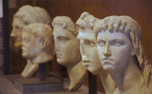

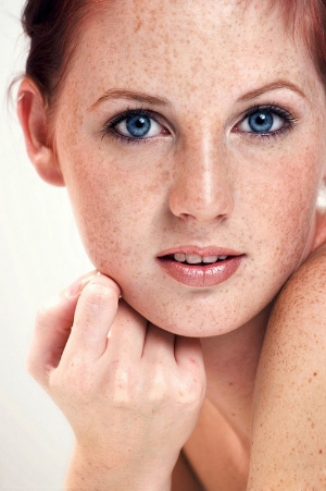
原图 半径3,ε=52


半径3,ε=102 半径3,ε=202

原图 半径5,ε=202
总体来说,P=G时,导向滤波的保边平滑特性和带有保边功能领域平滑滤波有类似的效果。

 浙公网安备 33010602011771号