语音合成最新进展
Tacotron2
前置知识
通过时域到频域的变换,可以得到从侧面看到的频谱,但是这个频谱并没有包含时域的中全部的信息,因为频谱只代表各个频率正弦波的振幅是多少,而没有提到相位。基础的正弦波\(Asin(wt+\theta)\)中,振幅、频率和相位缺一不可。不同相位决定了波的位置,所以对于频域分析,仅有频谱是不够的,还需要一个相位谱。
-
时域谱:时间-振幅
-
频域谱:频率-振幅
-
相位谱:相位-振幅
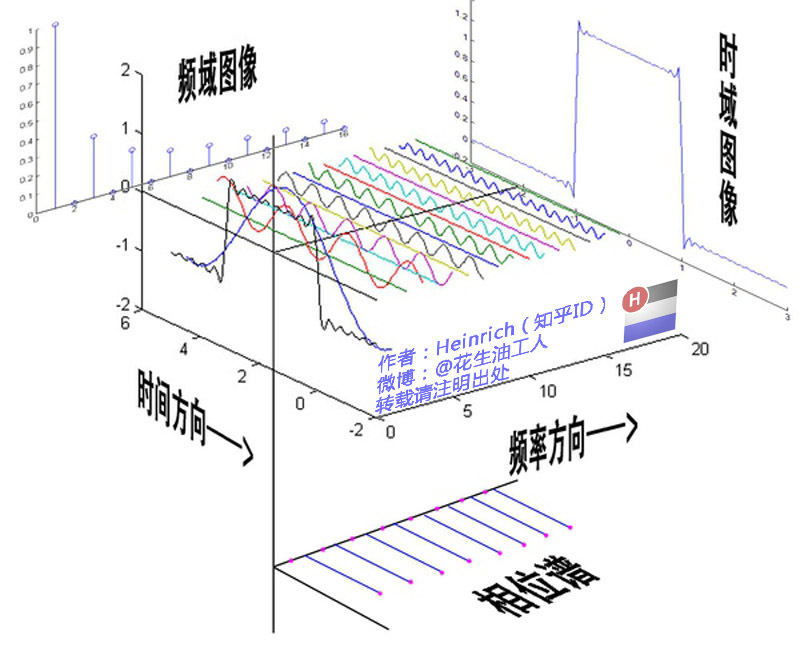
参见:傅里叶分析之掐死教程(完整版)更新于2014.06.06
传统语音合成:
- 单元挑选和拼接:将事先录制好的语音波形小片段缝合在一起。边界人工痕迹明显
- 统计参数:直接合成语音特征的平滑轨迹,交由声码器合成语音。发音模糊不清且不自然
Tacotron2分为两部分:
- 一个seq2seq结构的特征预测网络,将字符向量映射到梅尔声谱图
- 一个WaveNet修订版,将梅尔声谱图合成为时域波形
梅尔频谱是对短时傅里叶变换获得的声谱(即线性声谱)频率轴施加一个非线性变换,其依据人耳特性:低频细节对语音的理解十分关键,而高频细节可以淡化,对频率压缩变换而得。Tacotron2使用低层的声学特征梅尔声谱图来衔接两个部分的原因:
- 梅尔频谱容易通过时域波形计算得到
- 梅尔频谱对于每一帧都是相位不变的,容易使用均方差(MSE)训练
梅尔声谱抛弃了相位信息,而像Griffin-Lim算法对抛弃的相位信息进行估计,然后用一个短时傅里叶逆变换将梅尔声谱图转换为时域波形。可就是说,梅尔声谱是有损的,而声码器Griffin-Lim算法和近年出现的WaveNet有“找补”作用。Tacotron2特征预测网络选择梅尔频谱作为输出以减轻模型负担,再另加一个声码器WaveNet单独将梅尔频谱转波形。
声谱预测网络
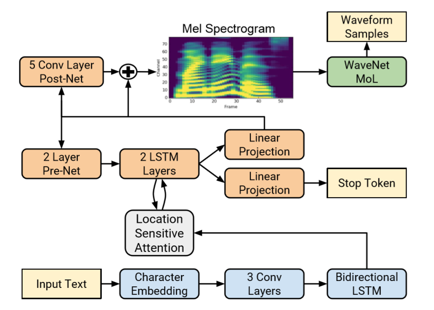
编码器将字符序列转化为一个隐状态,继而解码器接受隐状态用以预测声谱图。构建注意力网络用以消费编码器输出结果,编码器的每次输出,注意力网络都将编码序列归纳为上下文向量。最小化进入post-net前后的均方差以加速收敛。stop-token用于在推断(inference)时,动态结束生成过程。
WaveNet声码器
两部分组件分开训练,WaveNet依赖Tacotron2的特征预测网络的结果进行预测,一个替代方案是,使用从真实音频中抽取的梅尔频谱来训练WaveNet。注意:使用预测特征训练,就用预测特征推断;真实特征训练,真实特征推断;诸如使用预测特征训练,使用真实特征预测这种方法合成效果最差。
另外,论文中提到,梅尔频谱的通道数和合成语音质量是一种有趣的权衡;在解码后使用后处理网络结合上下文以改善合成质量,虽然WaveNet也含有卷积,但通过对比合成质量,加了后处理网络的合成质量更好些;与修改之前的30层卷积,256ms感受野的WaveNet相比,修改后的WaveNet卷积层减少到12层,感受野为10.5ms,但模型仍然合成了高质量的语音。因此对于语音质量来说,一个大的感受野并不是必须的,但是,如果去除所有的扩大卷积,感受野与基线模型相比小两个数量级,语音质量也大幅下降。因此虽然模型不需要一个大感受野,但是适当的上下文是必需的。
实现代码
以Tacotron-2_Rayhane-mamah@github为例,说明Tacotron2特征预测部分的实现。
特征预测网络的主文件位于Tacotron-2/tacotron/models/tacotron.py
-
Character Embedding,上图中,Input Text和Char Embedding:将Input Text映射到实数向量
[batch_size, sequence_length] -> [batch_size, sequence_length, embedding_size]
e.g.:
\[[ [2,4], [3] ]\\ \to \\ [[[0.3,0.1,0.5,0.9], [0.5,0.,1.9,0.3,0.4]], [[1.3,0.4,5.1,0.8]] \]embedding_table = tf.get_variable( 'inputs_embedding', [len(symbols), hp.embedding_dim], dtype=tf.float32) embedded_inputs = tf.nn.embedding_lookup(embedding_table, inputs)-
embedding_table: [len(symbols), embedding_size]. Tensorflow待训练变量,len(symbols)为所有字符的数目
-
inputs: [batch_size, sequence_length]. sequence_length为输入时间序列的步数,矩阵中的值为字符ID
-
embedded_inputs: [batch_size, sequence_length, embedding_size]
-
-
Encoder,上图中,3 Conv Layers和Bidirectional LSTM:编码器
[batch_size, sequece_length, embedding_size] -> [batch_size, encoder_steps, encoder_lstm_units]
encoder_cell = TacotronEncoderCell( EncoderConvolutions(is_training, hparams=hp, scope='encoder_convolutions'), EncoderRNN(is_training, size=hp.encoder_lstm_units, zoneout=hp.tacotron_zoneout_rate, scope='encoder_LSTM')) encoder_outputs = encoder_cell(embedded_inputs, input_lengths)-
encoder_outputs: [batch_size, encoder_steps, encoder_lstm_units]
其中,TacotronEncoderCell和BasicRNNCell、GRUCell、BasicLSTMCell一样,是自定义的RNNCell,继承自from tensorflow.contrib.rnn import RNNCell,参见:tensorflow中RNNcell源码分析以及自定义RNNCell的方法
- TacotronEncoderCell的参数之一EncoderConvolutions,对应于3 Conv Layers:
with tf.variable_scope(self.scope): x = inputs for i in range(self.enc_conv_num_layers): x = conv1d(x, self.kernel_size, self.channels, self.activation, self.is_training, self.drop_rate, 'conv_layer_{}_'.format(i + 1) + self.scope) return x- TacotronEncoderCell的参数之二EncoderRNN,对应于Bidirectional LSTM:
with tf.variable_scope(self.scope): outputs, (fw_state, bw_state) = tf.nn.bidirectional_dynamic_rnn( self._fw_cell, self._bw_cell, inputs, sequence_length=input_lengths, dtype=tf.float32, swap_memory=True) # Concat and return forward + backward outputs return tf.concat(outputs, axis=2)其中,self._fw_cell和self._bw_cell均为自定义的RNNCell,ZoneoutLSTMCell。这是一种最近出现的LSTM变种,参见:Zoneout: Regularizing RNNs by Randomly Preserving Hidden Activations
-
-
Decoder,上图中,2 Layer Pre-Net、Location Sensitive Attention、2 LSTM Layers和Linear Projection:解码器
[batch_size, encoder_steps, encoder_lstm_units] -> [batch_size, decoder_steps, num_mels×r]
# Attention Decoder Prenet prenet = Prenet(is_training, layers_sizes=hp.prenet_layers, drop_rate=hp.tacotron_dropout_rate, scope='decoder_prenet') # Attention Mechanism attention_mechanism = LocationSensitiveAttention(hp.attention_dim, encoder_outputs, hparams=hp, mask_encoder=hp.mask_encoder, memory_sequence_length=input_lengths, smoothing=hp.smoothing, cumulate_weights=hp.cumulative_weights) # Decoder LSTM Cells decoder_lstm = DecoderRNN(is_training, layers=hp.decoder_layers, size=hp.decoder_lstm_units, zoneout=hp.tacotron_zoneout_rate, scope='decoder_lstm')-
Prenet:2 Layer Pre-Net,Dense + Dropout
x = inputs with tf.variable_scope(self.scope): for i, size in enumerate(self.layers_sizes): dense = tf.layers.dense(x, units=size, activation=self.activation, name='dense_{}'.format(i + 1)) # The paper discussed introducing diversity in generation at inference time # by using a dropout of 0.5 only in prenet layers (in both training and inference). x = tf.layers.dropout(dense, rate=self.drop_rate, training=True, name='dropout_{}'.format(i + 1) + self.scope) return x -
LocationSensitiveAttention:Location Sensitive Attention
继承自from tensorflow.contrib.seq2seq.python.ops.attention_wrapper import BahdanauAttention的子类
Location Sensitive Attention是稍微改动的混合注意力机制:
-
energy
\[e_{ij}=v_a^Ttanh(Ws_i+Vh_j+Uf_{i,j}+b) \]其中,\(v_a^T\)、\(W\)、\(V\)、\(U\)和\(b\)为待训练参数,\(s_i\)为当前解码步上RNN隐状态,\(h_j\)为编码器隐状态,\(f_{i,j}\)经卷积的累加的之前的alignments
# processed_query shape [batch_size, query_depth] -> [batch_size, attention_dim] W_query = self.query_layer(query) if self.query_layer else query # -> [batch_size, 1, attention_dim] W_query = tf.expand_dims(processed_query, axis=1) # processed_location_features shape [batch_size, max_time, attention dimension] # [batch_size, max_time] -> [batch_size, max_time, 1] expanded_alignments = tf.expand_dims(previous_alignments, axis=2) # location features [batch_size, max_time, filters] f = self.location_convolution(expanded_alignments) # Projected location features [batch_size, max_time, attention_dim] W_fil = self.location_layer(f) v_a = tf.get_variable( 'attention_variable', shape=[num_units], dtype=dtype, initializer=tf.contrib.layers.xavier_initializer()) b_a = tf.get_variable( 'attention_bias', shape=[num_units], dtype=dtype, initializer=tf.zeros_initializer()) tf.reduce_sum(v_a * tf.tanh(W_keys + W_query + W_fil + b_a), axis=[2])其中,\(f_{i,j}\to W\_fil\):self.location_convolution & self.location_layer:
self.location_convolution = tf.layers.Conv1D(filters=hparams.attention_filters,
	kernel_size=hparams.attention_kernel, padding='same', use_bias=True,
	bias_initializer=tf.zeros_initializer(), name='location_features_convolution')

self.location_layer = tf.layers.Dense(units=num_units, use_bias=False,
	dtype=tf.float32, name='location_features_layer')
alignments | attention weights
\[\alpha_{ij}=\frac{exp(e_{ij})}{\sum_{k=1}^{T_x}exp(e_{ik})} \]alignments = self._probability_fn(energy, previous_alignments) -
context vector
\[c_{i}=\sum_{j=1}^{T_x}\alpha_{ij}h_j \]context = math_ops.matmul(expanded_alignments, attention_mechanism.values) context = array_ops.squeeze(context, axis=[1])
-
-
FrameProjection & StopProjection:Linear Projection,Dense
-
FrameProjection:
with tf.variable_scope(self.scope): #If activation==None, this returns a simple Linear projection #else the projection will be passed through an activation function # output = tf.layers.dense(inputs, units=self.shape, activation=self.activation, # name='projection_{}'.format(self.scope)) output = self.dense(inputs) return output -
StopProjection:
with tf.variable_scope(self.scope):
	output = tf.layers.dense(inputs, units=self.shape,
		activation=None, name='projection_{}'.format(self.scope))

	#During training, don't use activation as it is integrated inside the sigmoid_cross_entropy loss function
	if self.is_training:
		return output
	return self.activation(output)
-
-
在Decoder的实现中,将实例化的prenet、attention_mechanism、decoder_lstm、frame_projection和stop_projection传入TacotronDecoderCell:
decoder_cell = TacotronDecoderCell(
	prenet,
	attention_mechanism,
	decoder_lstm,
	frame_projection,
	stop_projection)
其中,TacotronDecoderCell继承自from tensorflow.contrib.rnn import RNNCell,
#Information bottleneck (essential for learning attention)
prenet_output = self._prenet(inputs)

#Concat context vector and prenet output to form LSTM cells input (input feeding)
LSTM_input = tf.concat([prenet_output, state.attention], axis=-1)

#Unidirectional LSTM layers
LSTM_output, next_cell_state = self._cell(LSTM_input, state.cell_state)


#Compute the attention (context) vector and alignments using
#the new decoder cell hidden state as query vector
#and cumulative alignments to extract location features
#The choice of the new cell hidden state (s_{i}) of the last
#decoder RNN Cell is based on Luong et Al. (2015):
#https://arxiv.org/pdf/1508.04025.pdf
previous_alignments = state.alignments
previous_alignment_history = state.alignment_history
context_vector, alignments, cumulated_alignments = _compute_attention(self._attention_mechanism,
	LSTM_output,
	previous_alignments,
	attention_layer=None)

#Concat LSTM outputs and context vector to form projections inputs
projections_input = tf.concat([LSTM_output, context_vector], axis=-1)

#Compute predicted frames and predicted <stop_token>
cell_outputs = self._frame_projection(projections_input)
stop_tokens = self._stop_projection(projections_input)

#Save alignment history
alignment_history = previous_alignment_history.write(state.time, alignments)

#Prepare next decoder state
next_state = TacotronDecoderCellState(
	time=state.time + 1,
	cell_state=next_cell_state,
	attention=context_vector,
	alignments=cumulated_alignments,
	alignment_history=alignment_history)

return (cell_outputs, stop_tokens), next_state
然后定义helper,初始化后,开始解码:
#Define the helper for our decoder
if is_training or is_evaluating or gta:
	self.helper = TacoTrainingHelper(batch_size, mel_targets, stop_token_targets, hp, gta, is_evaluating, global_step)
else:
	self.helper = TacoTestHelper(batch_size, hp)


#initial decoder state
decoder_init_state = decoder_cell.zero_state(batch_size=batch_size, dtype=tf.float32)

#Only use max iterations at synthesis time
max_iters = hp.max_iters if not (is_training or is_evaluating) else None

#Decode
(frames_prediction, stop_token_prediction, _), final_decoder_state, _ = dynamic_decode(
	CustomDecoder(decoder_cell, self.helper, decoder_init_state),
	impute_finished=False,
	maximum_iterations=max_iters,
	swap_memory=hp.tacotron_swap_with_cpu)


# Reshape outputs to be one output per entry
#==> [batch_size, non_reduced_decoder_steps (decoder_steps * r), num_mels]
decoder_output = tf.reshape(frames_prediction, [batch_size, -1, hp.num_mels])
stop_token_prediction = tf.reshape(stop_token_prediction, [batch_size, -1])
Seq2Seq定义简明说明参见:Tensorflow新版Seq2Seq接口使用、Dynamic Decoding-Tensorflow
-
Postnet,上图中,5 Conv Layer Post-Net:后处理网络
[batch_size, decoder_steps, num_mels×r] -> [batch_size, decoder_steps×r, postnet_channels]
with tf.variable_scope(self.scope):
	x = inputs
	for i in range(self.postnet_num_layers - 1):
		x = conv1d(x, self.kernel_size, self.channels, self.activation,
			self.is_training, self.drop_rate, 'conv_layer_{}_'.format(i + 1)+self.scope)
	x = conv1d(x, self.kernel_size, self.channels, lambda _: _, self.is_training, self.drop_rate,
		'conv_layer_{}_'.format(5)+self.scope)
return x
之后进入残差部分:
[batch_size, decoder_steps×r, postnet_channels] -> [batch_size, decoder_steps×r, num_mels]
residual_projection = Dense(hp.num_mels, scope='postnet_projection')
projected_residual = residual_projection(residual)

mel_outputs = decoder_output + projected_residual
此外,代码中还提供了“开关”后处理CBHG的选项:
if post_condition: # Add post-processing CBHG: post_outputs = post_cbhg(mel_outputs, hp.num_mels, is_training) # [N, T_out, 256] linear_outputs = tf.layers.dense(post_outputs, hp.num_freq) -
Loss计算
self.loss = self.before_loss + self.after_loss + self.stop_token_loss + self.regularization_loss + self.linear_loss-
self.before_loss & self.after_loss
送入Post-Net前的MaskedMSE & 经过Post-Net和残差之后的MaskedMSE,MaskedMSE定义如下:
def MaskedMSE(targets, outputs, targets_lengths, hparams, mask=None):
	'''Computes a masked Mean Squared Error
	'''

	#[batch_size, time_dimension, 1]
	#example:
	#sequence_mask([1, 3, 2], 5) = [[[1., 0., 0., 0., 0.]],
	#							    [[1., 1., 1., 0., 0.]],
	#							    [[1., 1., 0., 0., 0.]]]
	#Note the maxlen argument that ensures mask shape is compatible with r>1
	#This will by default mask the extra paddings caused by r>1
	if mask is None:
		mask = sequence_mask(targets_lengths, hparams.outputs_per_step, True)

	#[batch_size, time_dimension, channel_dimension(mels)]
	ones = tf.ones(shape=[tf.shape(mask)[0], tf.shape(mask)[1], tf.shape(targets)[-1]], dtype=tf.float32)
	mask_ = mask * ones

	with tf.control_dependencies([tf.assert_equal(tf.shape(targets), tf.shape(mask_))]):
		return tf.losses.mean_squared_error(labels=targets, predictions=outputs, weights=mask_)
即:在计算预测和Ground-Truth序列的均方差时,对超过Ground-Truth长度处的方差置0。
-
self.stop_token_loss
Ground-Truth的stop-token概率和预测的stop-token概率两者的交叉熵,stop-token是通过一个简单的逻辑回归预测,超过0.5则停止序列生成。和MaskedMSE类似,MaskedSigmoidCrossEntropy定义如下:
def MaskedSigmoidCrossEntropy(targets, outputs, targets_lengths, hparams, mask=None): '''Computes a masked SigmoidCrossEntropy with logits ''' #[batch_size, time_dimension] #example: #sequence_mask([1, 3, 2], 5) = [[1., 0., 0., 0., 0.], # [1., 1., 1., 0., 0.], # [1., 1., 0., 0., 0.]] #Note the maxlen argument that ensures mask shape is compatible with r>1 #This will by default mask the extra paddings caused by r>1 if mask is None: mask = sequence_mask(targets_lengths, hparams.outputs_per_step, False) with tf.control_dependencies([tf.assert_equal(tf.shape(targets), tf.shape(mask))]): #Use a weighted sigmoid cross entropy to measure the <stop_token> loss. Set hparams.cross_entropy_pos_weight to 1 #will have the same effect as vanilla tf.nn.sigmoid_cross_entropy_with_logits. losses = tf.nn.weighted_cross_entropy_with_logits(targets=targets, logits=outputs, pos_weight=hparams.cross_entropy_pos_weight) with tf.control_dependencies([tf.assert_equal(tf.shape(mask), tf.shape(losses))]): masked_loss = losses * mask return tf.reduce_sum(masked_loss) / tf.count_nonzero(masked_loss, dtype=tf.float32) -
self.regularization_loss
所有变量的正则化Loss
# Get all trainable variables all_vars = tf.trainable_variables() regularization = tf.add_n([tf.nn.l2_loss(v) for v in all_vars if not ('bias' in v.name or 'Bias' in v.name)]) * reg_weight -
self.linear_loss
当特征网络预测线性谱时,特有的Loss。特别加大低于2000Hz线性谱的Ground-Truth和预测的Loss,这是因为低频对理解音频十分重要
def MaskedLinearLoss(targets, outputs, targets_lengths, hparams, mask=None): '''Computes a masked MAE loss with priority to low frequencies ''' #[batch_size, time_dimension, 1] #example: #sequence_mask([1, 3, 2], 5) = [[[1., 0., 0., 0., 0.]], # [[1., 1., 1., 0., 0.]], # [[1., 1., 0., 0., 0.]]] #Note the maxlen argument that ensures mask shape is compatible with r>1 #This will by default mask the extra paddings caused by r>1 if mask is None: mask = sequence_mask(targets_lengths, hparams.outputs_per_step, True) #[batch_size, time_dimension, channel_dimension(freq)] ones = tf.ones(shape=[tf.shape(mask)[0], tf.shape(mask)[1], tf.shape(targets)[-1]], dtype=tf.float32) mask_ = mask * ones l1 = tf.abs(targets - outputs) n_priority_freq = int(2000 / (hparams.sample_rate * 0.5) * hparams.num_freq) with tf.control_dependencies([tf.assert_equal(tf.shape(targets), tf.shape(mask_))]): masked_l1 = l1 * mask_ masked_l1_low = masked_l1[:,:,0:n_priority_freq] mean_l1 = tf.reduce_sum(masked_l1) / tf.reduce_sum(mask_) mean_l1_low = tf.reduce_sum(masked_l1_low) / tf.reduce_sum(mask_) return 0.5 * mean_l1 + 0.5 * mean_l1_low可以阅读hp.mask_decoder == False时的Loss计算,即不对decoder进行Mask,更容易理解计算整个网络Loss的方法。
-
-
优化
使用AdamOptimizer优化,值得注意的是,默认学习率策略:
-
< 50k steps: lr = 1e-3
-
[50k, 310k] steps: lr = 1e-3 ~ 1e-5,指数下降:tf.train.exponential_decay
-
> 310 k steps: lr = 1e-5
# Compute natural exponential decay
lr = tf.train.exponential_decay(learning_rate = init_lr,
								global_step = global_step - hp.tacotron_start_decay,  # lr = 1e-3 at step 50k
								decay_steps = self.decay_steps,
								decay_rate = self.decay_rate,  # lr = 1e-5 around step 310k
								name='lr_exponential_decay')

# clip learning rate by max and min values (initial and final values)
return tf.minimum(tf.maximum(lr, hp.tacotron_final_learning_rate), init_lr)
学习率指数衰减:
decayed_learning_rate=learining_rate*decay_rate^(global_step/decay_steps)
-
ClariNet
ClariNet改进重点在WaveNet。论文地址:ClariNet: Parallel Wave Generation in End-to-End Text-to-Speech
论文贡献:
- 单高斯简化parallel WaveNet的KL目标函数,改进了蒸馏法(distillation)算法,使得结构更简单,更稳定
- 通过Bridge-net连接了Tacotron(特征预测网络)和WaveNet,彻底端到端
前置知识
-
KL散度
\[\begin{align*} KL(P||Q)&=\int_{-\infty }^{+\infty}p(x)log\frac{p(x)}{q(x)}dx\\ &=\int_{-\infty}^{+\infty}p(x)logp(x)-\int_{-\infty}^{+\infty}p(x)logq(x)\\ &=-H(P)+H(P,Q) \end{align*} \]其中,\(-H(P)\)为固定值,\(H(P,Q)\)为交叉熵。最小化\(KL(P||Q)\),等价于最小化交叉熵。散度是差值的意思,散度越小,两个分布越相像。
KL散度是非负的,这种度量是不对称的,也即是\(KL(P||Q)\neq KL(Q||P)\)
![]()
现在希望使用简单分布\(q\)拟合复杂分布\(p\),使用\(KL(q||p)\)做最优化,是希望p(x)为0的地方q(x)也为0,否则
\(\frac{q(x)}{p(x)}\)会很大(上图中右侧两张图);使用\(KL(p||q)\)做最优化,就是尽量避免p(x)不为0而q(x)用0去拟合,上图中最左侧的图。因此,\(KL(q||p)\)得到的近似分布\(q(x)\)会比较窄,因为其希望\(q(x)\)为0的地方比较多(上图右侧两图);而\(KL(p||q)\)得到的近似分布\(q(x)\)会比较宽,因为其希望\(q(x)\)为0的地方比较多(上图最左侧图)。
由于\(KL(q||p)\)至少可以拟合到其中一个峰上,而\(KL(p||q)\)拟合的结果,其概率密度最大的地方可能没有什么意义,因此在通常情况下,使用简单分布\(q\)拟合复杂分布\(p\)时,\(KL(q||p)\)更符合我们的需要。
-
变分推断
变分推断的核心思想是:用形式简单的分布去近似形式复杂、不易计算的分布。比如,我们可以在指数族函数空间当中,选一个和目标分布最相像的分布,这样计算起来就方便多了。所谓“变分”,就是从函数空间中找到满足某些条件或约束的函数。
参见:PRML读书会第十章 Approximate Inference(近似推断,变分推断,KL散度,平均场, Mean Field )

之前的WaveNet可以根据任意形式的输入直接合成波形,结构是纯卷积的,没有循环层,在训练时可以在采样点的级别上并行,效率很高;但是在预测时是自回归的,即每个采样点都依赖于之前的采样点,效率很低。
这里构建“学生”和“老师”两种网络,作为学生的网络一般比老师的网络结构更简单,但是希望凭借学生这种简单的结构学到老师的精华,这种在网络间传授知识的过程称作“蒸馏”(distill)。一般来说,蒸馏的过程是让学生网络的输出分布尽可能逼近老师网络的输出分布,这一般是通过最小化两个网络输出分布之间的KL散度实现的。
之前WaveNet的输出层是一个分类层,输出0~255的离散样本值,这不适合从老师传授给学生,于是parallel WaveNet的作者们将输出改造为连续的mixture of logistics(MoL)分布,而学生网络的输出分布使用的是logistic inverse auto-regressive flow,学生网络虽然也称“auto-regressive”,但实际上合成是并行的。parallel WaveNet的蒸馏过程使用了大量的logistic函数,这导致学生网络和老师网络的输出分布的KL散度很难计算,不得不用蒙特卡洛方法近似,于是网络的蒸馏过程容易出现数值不稳定的情况。
ClariNet将老师的输出分布简化为单高斯分布,并通过实验证明这并不影响合成效果。学生的输出分布改为了高斯逆回归流(Gaussian IAF),简化的好处在于两边输出分布的KL散度能够写出显式表达式,蒸馏过程可以通过正常的梯度下降法来完成。
论文中,使用一种改进的KL散度衡量学生和老师网络输出分布的差异:

 浙公网安备 33010602011771号