
Comprehensive Guide to build a Recommendation Engine from scratch (in Python) / 从0开始搭建推荐系统
https://www.analyticsvidhya.com/blog/2018/06/comprehensive-guide-recommendation-engine-python/, 一篇详细的入门级的推荐系统的文章,这篇文章内容详实,格式漂亮,推荐给大家.
下面是翻译,翻译关注的是意思,不是直译哈,大家将就着看, 如果英文好,推荐看原文,原文的排版比我这个舒服多了.
NOTE: 原文中发现一个有误的地方,下面我会用 红色 标出来. 同时,我在翻译的过程中,有疑虑或者值得商榷的地方,我会用 蓝色 标出来.
Comprehensive Guide to build a Recommendation Engine from scratch (in Python)
从0开始搭建推荐系统
Introduction / 简介
In today’s world, every customer is faced with multiple choices. For example, If I’m looking for a book to read without any specific idea of what I want, there’s a wide range of possibilities how my search might pan out. I might waste a lot of time browsing around on the internet and trawling through various sites hoping to strike gold. I might look for recommendations from other people.
现如今,每个顾客都面临多种选择. 比如,假如我想读书又不知道看点什么,那就有无数种可能的选择。我可能会浪费大把的时间在网上搜索或者盲目地在各个书店撒网希望淘到喜欢的书。我也可能需求其他人的推荐.
But if there was a site or app which could recommend me books based on what I have read previously, that would be a massive help. Instead of wasting time on various sites, I could just log in and voila! 10 recommended books tailored to my taste.
但是如果有这么一个网站或者APP能基于我以前读过什么来给我推荐书籍,那该多好啊. 我不是在各个网站浪费时间,而是直接找到10本满足我口味的书细细品味.

This is what recommendation engines do and their power is being harnessed by most businesses these days. From Amazon to Netflix, Google to Goodreads, recommendation engines are one of the most widely used applications of machine learning techniques.
这就是推荐引擎要做的事情,并且它的功用也得到的大多数商业行为的使用. 从 Amazon 到 Netfix, Google 到 Goodreads, 推荐引擎成为了最常见的机器学习技术的一种.
In this article, we will cover various types of recommendation engine algorithms and fundamentals of creating them in Python. We will also see the mathematics behind the workings of these algorithms. Finally, we will create our own recommendation engine using matrix factorization.
在这篇文章里,我们将讲到各种不同的推荐引擎算法和原理并用python 创建他们. 我们也将看到这些算法背后的数学知识. 最后,我们将用 matrix factorization 来创建我们自己的推荐引擎.
Table of Contents 目录
- What are recommendation engines? 什么是推荐引擎
- How does a recommendation engine work? 推荐引擎是怎么工作的Case study in Python using the MovieLens dataset 基于MovieLens数据集用python实现的案例
- Data collection 数据收集
- Data storage 数据存储 Filtering the data 数据过滤
- Content based filtering 基于内容的过滤
- Collaborative filtering 协同过滤
- Case study in Python using the MovieLens dataset / 基于MovieLens 数据集的案例学习python实现
- Building collaborative filtering model from scratch / 从0开始创建协同过滤模型
- Building Simple popularity and collaborative filtering model using Turicreate / 使用 Turicreate 创建简单的基于欢迎度的模型和协同过滤模型
- Introduction to matrix factorization / 介绍 matrix factorization
- Building a recommendation engine using matrix factorization / 使用 matrix factorization 创建推荐引擎 Evaluation metrics for recommendation engines / 推荐引擎效果评估
- Recall
- Precision
- RMSE (Root Mean Squared Error)
- Mean Reciprocal Rank
- MAP at k (Mean Average Precision at cutoff k)
- NDCG (Normalized Discounted Cumulative Gain)
- What else can be tried? / 其他有哪些可以尝试?
1. What are recommendation engines? / 推荐引擎是什么?
Till recently, people generally tended to buy products recommended to them by their friends or the people they trust. This used to be the primary method of purchase when there was any doubt about the product. But with the advent of the digital age, that circle has expanded to include online sites that utilize some sort of recommendation engine.
人们一般倾向于在买东西时寻求他们的朋友或者他们相信的人推荐的产品. 这是过去最常见的购买方式尤其是当他们对要买的产品有疑虑时. 但是随着数字时代的到来,这个过程就包含了使用推荐引擎来在线的推荐产品.
A recommendation engine filters the data using different algorithms and recommends the most relevant items to users. It first captures the past behavior of a customer and based on that, recommends products which the users might be likely to buy.
推荐引擎使用不同的算法过滤数据,并推荐给用户最相关的东西. 它捕捉客户的历史行为,并且基于这些历史行为给用户推荐他们最可能买的东西.
If a completely new user visits an e-commerce site, that site will not have any past history of that user. So how does the site go about recommending products to the user in such a scenario? One possible solution could be to recommend the best selling products, i.e. the products which are high in demand. Another possible solution could be to recommend the products which would bring the maximum profit to the business.
如果是一个全新的用户访问电商网站,这个站点没有这个用户的任何历史信息. 那么这种情况下网站怎么推荐呢?一个可能的方案是推荐热销的商品,比如,高需求量的商品; 另一个方案是推荐那些给公司带来高收益的产品.
If we can recommend a few items to a customer based on their needs and interests, it will create a positive impact on the user experience and lead to frequent visits. Hence, businesses nowadays are building smart and intelligent recommendation engines by studying the past behavior of their users.
如果我们能根据用户的需求和兴趣推荐一些产品给他们,这将产生有益的效果并且带来更多的访问. 因此,现代商业活动正在基于他们用户的行为建立只能推荐引擎.
Now that we have an intuition of recommendation engines, let’s now look at how they work.
现在我们对推荐引擎有了一个直观的认识,让我们来看看它是怎么工作的
2. How does a recommendation engine work? / 推荐引擎怎么工作的?
Before we deep dive into this topic, first we’ll think of how we can recommend items to users:
在我们深入研究之前,我们先想一下我们怎么推荐产品给用户
- We can recommend items to a user which are most popular among all the users / 我们可以给所有用户推荐正在热销的产品
- We can divide the users into multiple segments based on their preferences (user features) and recommend items to them based on the segment they belong to / 我们也可以按照用户的喜好特征把用户分组,然后按照分组分别推荐不同的东西给他们
Both of the above methods have their drawbacks. In the first case, the most popular items would be the same for each user so everybody will see the same recommendations. While in the second case, as the number of users increases, the number of features will also increase. So classifying the users into various segments will be a very difficult task.
以上两种方法都有缺陷.第一种方法,所有人都收到的是一样的产品的推荐. 第二种方法,如果用户不断增加,用户的喜好特征也会增加,再次给用户归类是一个困难的工作.
The main problem here is that we are unable to tailor recommendations based on the specific interest of the users. It’s like Amazon is recommending you buy a laptop just because it’s been bought by the majority of the shoppers. But thankfully, Amazon (or any other big firm) does not recommend products using the above mentioned approach. They use some personalized methods which help them in recommending products more accurately.
这里的主要问题是我们不能根据用户各自的兴趣来定制化的推荐. 就像Amanzon 因为其他很多人买了笔记本电脑也给你推荐了笔记本电脑. 但是幸运的是,Amazon并不是这样推荐的, 他们使用的个性化的推荐方法,这样的推荐更加精确.
Let’s now focus on how a recommendation engine works by going through the following steps.
现在我们更深入的按步骤讲解推荐引擎的工作方式.
2.1 Data collection / 数据收集
This is the first and most crucial step for building a recommendation engine. The data can be collected by two means: explicitly and implicitly. Explicit data is information that is provided intentionally, i.e. input from the users such as movie ratings. Implicit data is information that is not provided intentionally but gathered from available data streams like search history, clicks, order history, etc.
这是创建推荐引擎第一步也是最重要的一步。两种方法可以收集收据:明采和暗采。明采就是让用户主动输入反馈,比如对所购商品的评价打分;暗采就是系统在前台收集后台记录用户的行为数据,常见的有用户的鼠标点击行为,搜索记录, 购买记录等.
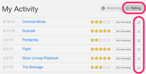
In the above image, Netflix is collecting the data explicitly in the form of ratings given by user to different movies.
上图中,Netfix 使用的就用明采的方法让用户主动给电影打分评级.

Here the order history of a user is recorded by Amazon which is an example of implicit mode of data collection.
这是一个Amazon 网站的用户购买记录,属于暗采方法.
2.2 Data storage / 数据存储
The amount of data dictates how good the recommendations of the model can get. For example, in a movie recommendation system, the more ratings users give to movies, the better the recommendations get for other users. The type of data plays an important role in deciding the type of storage that has to be used. This type of storage could include a standard SQL database, a NoSQL database or some kind of object storage.
数据量的多少会影响推荐模型的精度. 比如,一个电影推荐系统,用户给的打分越多,推荐就会越准确. 数据的类型决定了存储类型. 存储类型有标准的SQL数据库,NoSQL 数据库和对象存储.
2.3 Filtering the data / 数据过滤
After collecting and storing the data, we have to filter it so as to extract the relevant information required to make the final recommendations.
收集到数据并存储好以后,我们要过滤数据来找到相关信息,然后做出最终推荐.

Source: intheshortestrun
There are various algorithms that help us make the filtering process easier. In the next section, we will go through each algorithm in detail.
有各种各样的算法可以帮我们的过滤流程更加容易. 接下来,我们就一个一个来看看.
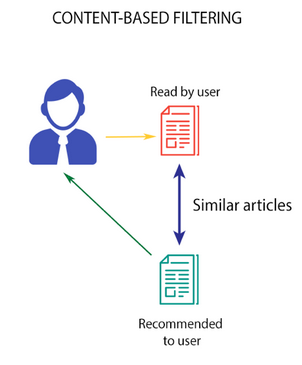
2.3.1 Content based filtering / 基于内容的过滤
This algorithm recommends products which are similar to the ones that a user has liked in the past.
这个算法推荐给用户那些他以前喜欢过的东西的类似产品.
Source: Medium
For example, if a person has liked the movie “Inception”, then this algorithm will recommend movies that fall under the same genre. But how does the algorithm understand which genre to pick and recommend movies from?
比如,如果一个人喜欢电影《盗梦空间》,那么这个算法就会推荐相同类型的电影. 但是,这个算法怎么知道根据电影的哪个属性来推荐呢?
Consider the example of Netflix. They save all the information related to each user in a vector form. This vector contains the past behavior of the user, i.e. the movies liked/disliked by the user and the ratings given by them. This vector is known as the profile vector. All the information related to movies is stored in another vector called the item vector. Item vector contains the details of each movie, like genre, cast, director, etc.
考虑Netflix 的例子,他们保存了所有的用户信息在向量里,这个向量包含了这个用户的过往行为,比如他喜欢或者不喜欢那些电影,给电影评了多少分. 这个向量叫做用户属性向量。所有与电影本身相关的属性,比如电影类型,导演,年代信息等会保存在另一个向量里,叫产品属性向量.
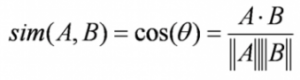
The content-based filtering algorithm finds the cosine of the angle between the profile vector and item vector, i.e. cosine similarity. Suppose A is the profile vector and B is the item vector, then the similarity between them can be calculated as:
基于内容的过滤算法找出用户属性向量和产品属性向量的夹角的cos值,比如 cos 相似性. 假如A是用户属性向量,B是产品属性向量,他们两者的相似性可以计算如下:
(译者注:我觉得A和B是两种完全不同的类型,不应该去计算相似性,这里值得商榷)
Based on the cosine value, which ranges between -1 to 1, the movies are arranged in descending order and one of the two below approaches is used for recommendations:
基于cos值(-1 ~ 1),把电影按照从大到小的值排列,然后使用下面两种方法推荐:
- Top-n approach: where the top n movies are recommended (Here n can be decided by the business) / 推荐最大的几个,至于是几个,取决于业务需求
- Rating scale approach: Where a threshold is set and all the movies above that threshold are recommended / 设定一个阈值,凡是>阈值的都推荐
Other methods that can be used to calculate the similarity are: / 除了cos相似性,其他计算相似性的方法有:
- Euclidean Distance: Similar items will lie in close proximity to each other if plotted in n-dimensional space. So, we can calculate the distance between items and based on that distance, recommend items to the user. The formula for the euclidean distance is given by: / 欧几里得距离: 没啥说头,自己看公式
![]()
- Pearson’s Correlation: It tells us how much two items are correlated. Higher the correlation, more will be the similarity. Pearson’s correlation can be calculated using the following formula: / Pearson相关性(译者注:我理解就是cos相关性的一个变种,先求mean,在算cos 相似性,为的是消除人为喜好造成的参数分布差异,比如有些人容易满足对产品总是打高分,有些人比较挑剔容易打低分)

A major drawback of this algorithm is that it is limited to recommending items that are of the same type. It will never recommend products which the user has not bought or liked in the past. So if a user has watched or liked only action movies in the past, the system will recommend only action movies. It’s a very narrow way of building an engine.
这个算法主要的缺点是只能推荐用户买过的相似的东西。如果用户没有买过东西,那就无能为力了. 如果用户只看过动作片,那么它就只会推动作片给用户. 这种推荐相对比较low.
To improve on this type of system, we need an algorithm that can recommend items not just based on the content, but the behavior of users as well.
为了改善这个系统,我们需要一个算法,既能基于内容,也能基于用户行为来推荐.
2.3.2 Collaborative filtering / 协同过滤
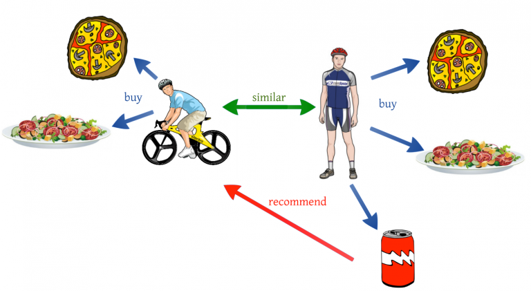
Let us understand this with an example. If person A likes 3 movies, say Interstellar, Inception and Predestination, and person B likes Inception, Predestination and The Prestige, then they have almost similar interests. We can say with some certainty that A should like The Prestige and B should like Interstellar. The collaborative filtering algorithm uses “User Behavior” for recommending items. This is one of the most commonly used algorithms in the industry as it is not dependent on any additional information. There are different types of collaborating filtering techniques and we shall look at them in detail below.
举一个例子来理解. 如果一个人A喜欢3个电影 <星际>,<盗梦空间>,和<前目的地>, 另一个人B喜欢<盗梦空间>,<前目的地>和<致命魔术>. 我们一定程度上可以说A应该会喜欢<致命魔术>,B应该会喜欢<星际>. 协同过滤使用“用户行为“来推荐. 这是业界常用的算法因为他不依赖与任何其他信息. 有几种不同的协同过滤技术,我们接下来仔细来了解下.
User-User collaborative filtering / 用户-用户 协同过滤
This algorithm first finds the similarity score between users. Based on this similarity score, it then picks out the most similar users and recommends products which these similar users have liked or bought previously.
这个算法先找到用户之间的相似性. 基于这个相似性数据,给用户推荐那些和他有最像的行为的用户买过的东西.
Source: Medium
In terms of our movies example from earlier, this algorithm finds the similarity between each user based on the ratings they have previously given to different movies. The prediction of an item for a user u is calculated by computing the weighted sum of the user ratings given by other users to an item i.
根据我们之前的电影例子,这个算法找出给过评分的用户的相似性. 用户u 给商品 i 打分的预测公式如下:
The prediction Pu,i is given by:

Here, / 这里
- Pu,i is the prediction of an item / 用户u 给商品 i 评分的预测值
- Rv,i is the rating given by a user v to a movie i
- Su,v is the similarity between users
Now, we have the ratings for users in profile vector and based on that we have to predict the ratings for other users. Following steps are followed to do so:
现在,我们有了用户属性向量,基于这个我们就可以做预测了. 具体步骤如下:
- For predictions we need the similarity between the user u and v. We can make use of Pearson correlation. / 我们选的是Pearson相关性
- First we find the items rated by both the users and based on the ratings, correlation between the users is calculated. / 那就算吧
- The predictions can be calculated using the similarity values. This algorithm, first of all calculates the similarity between each user and then based on each similarity calculates the predictions. Users having higher correlation will tend to be similar. / 算出一个大的矩阵,矩阵里面的数字越接近1,越相似.
- Based on these prediction values, recommendations are made. Let us understand it with an example: / 下面例子讲的很清楚
Consider the user-movie rating matrix:
这是一个user-movie 矩阵:
| User/Movie | x1 | x2 | x3 | x4 | x5 | Mean User Rating |
| A | 4 | 1 | – | 4 | – | 3 |
| B | – | 4 | – | 2 | 3 | 3 |
| C | – | 1 | – | 4 | 4 | 3 |
Here we have a user movie rating matrix. To understand this in a more practical manner, let’s find the similarity between users (A, C) and (B, C) in the above table. Common movies rated by A/[ and C are movies x2 and x4 and by B and C are movies x2, x4 and x5.
A和C对电影x2,x4 都打分了,B和C对 x2,x4,x5 都打分了. 下面的算式pearson 相关性算式.

The correlation between user A and C is more than the correlation between B and C. Hence users A and C have more similarity and the movies liked by user A will be recommended to user C and vice versa.
可以看出, A 和C相关性很高,如果A喜欢什么,那就推荐给C. 相反亦然.
This algorithm is quite time consuming as it involves calculating the similarity for each user and then calculating prediction for each similarity score. One way of handling this problem is to select only a few users (neighbors) instead of all to make predictions, i.e. instead of making predictions for all similarity values, we choose only few similarity values. There are various ways to select the neighbors:
这个算法非常耗时间因为它要先计算相似性矩阵然后计算预测值. 一个解决这个问题的方法是求出相似度矩阵后选择一部分邻居用户来计算预测值.
- Select a threshold similarity and choose all the users above that value / 把相似性大于一定阈值的的用户选进来
- Randomly select the users / 随机选用户
- Arrange the neighbors in descending order of their similarity value and choose top-N users / 选前几个最相似的用户
- Use clustering for choosing neighbors / 使用聚类算法找邻居用户
This algorithm is useful when the number of users is less. Its not effective when there are a large number of users as it will take a lot of time to compute the similarity between all user pairs. This leads us to item-item collaborative filtering, which is effective when the number of users is more than the items being recommended.
这个算法如果用户数量少还可以,如果用户太多了,相似性矩阵就会很大,计算量太大,所有如果用户数量大于商品数量的情况下,采用的是接下来讲到的 产品-产品 协同过滤.
Item-Item collaborative filtering / 产品-产品协同过滤
In this algorithm, we compute the similarity between each pair of items.
这个算法,我们技术产品之间的相似性
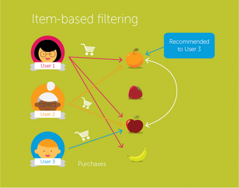
Source: Medium
So in our case we will find the similarity between each movie pair and based on that, we will recommend similar movies which are liked by the users in the past. This algorithm works similar to user-user collaborative filtering with just a little change – instead of taking the weighted sum of ratings of “user-neighbors”, we take the weighted sum of ratings of “item-neighbors”. The prediction is given by:
基本思想是,你喜欢过一种商品,那就把相似的商品推给你. 预测公式如下.

Now we will find the similarity between items. / 相似性用cos 相似性

Now, as we have the similarity between each movie and the ratings, predictions are made and based on those predictions, similar movies are recommended. Let us understand it with an example. / 看例子很清楚
| User/Movie | x1 | x2 | x3 | x4 | x5 |
| A | 4 | 1 | 2 | 4 | 4 |
| B | 2 | 4 | 4 | 2 | 1 |
| C | – | 1 | – | 3 | 4 |
| Mean Item Rating | 3 | 2 | 3 | 3 | 3 |
Here the mean item rating is the average of all the ratings given to a particular item (compare it with the table we saw in user-user filtering). Instead of finding the user-user similarity as we saw earlier, we find the item-item similarity.
To do this, first we need to find such users who have rated those items and based on the ratings, similarity between the items is calculated. Let us find the similarity between movies (x1, x4) and (x1, x5). Common users who have rated movies x1 and x4 are A and B while the users who have rated movies x1 and x5 are also A and B.
(译者注: 本来说好用 cos 相似性的,结果作者忽悠我们,他用了 pearson 相似性,因为每个数组都借去了mean. 其实没必要, 直接cos相似性就挺好.)

The similarity between movie x1 and x4 is more than the similarity between movie x1 and x5. So based on these similarity values, if any user searches for movie x1, they will be recommended movie x4 and vice versa. Before going further and implementing these concepts, there is a question which we must know the answer to – what will happen if a new user or a new item is added in the dataset? It is called a Cold Start. There can be two types of cold start:
这里有个有意思的概念注意一下,叫冷启动,就是一个新用户和新产品加入了我们的系统
- Visitor Cold Start
- Product Cold Start
Visitor Cold Start means that a new user is introduced in the dataset. Since there is no history of that user, the system does not know the preferences of that user. It becomes harder to recommend products to that user. So, how can we solve this problem? One basic approach could be to apply a popularity based strategy, i.e. recommend the most popular products. These can be determined by what has been popular recently overall or regionally. Once we know the preferences of the user, recommending products will be easier.
新用户加入,我不知道你的过往行为,那就可以给你推送最近流行的产品
On the other hand, Product Cold Start means that a new product is launched in the market or added to the system. User action is most important to determine the value of any product. More the interaction a product receives, the easier it is for our model to recommend that product to the right user. We can make use of Content based filtering to solve this problem. The system first uses the content of the new product for recommendations and then eventually the user actions on that product.
新产品加入,我不知道你和其他产品的相似性,那就人工来标注新产品的属性,比如给产品打上日用品,家电等标签,然后基于内容推送, 有人正在关注家电那就推荐给他.
Now let’s solidify our understanding of these concepts using a case study in Python. Get your machines ready because this is going to be fun!
现在我们通过python 的例子来加深理解. 准备好机器,开干吧!
3. Case study in Python using the MovieLens Dataset / 基于MovieLens数据集的案例学习,使用python语言
We will work on the MovieLens dataset and build a model to recommend movies to the end users. This data has been collected by the GroupLens Research Project at the University of Minnesota. The dataset can be downloaded from here. This dataset consists of:
我们将基于明尼苏达大学的GroupLens 研究项目采集的MovieLens数据集来创建一个模型. 这个数据集有943个用户1682个电影的数据,总共100k的rating 数据. 数据集可以在这里下载
- 100,000 ratings (1-5) from 943 users on 1682 movies
- Demographic information of the users (age, gender, occupation, etc.)
First, we’ll import our standard libraries and read the dataset in Python.
首先,导入python常用库并读取数据集
import pandas as pd
%matplotlib inline
import matplotlib
import matplotlib.pyplot as plt
import numpy as np

# pass in column names for each CSV as the column name is not given in the file and read them using pandas.
# You can check the column names from the readme file

#Reading users file:
u_cols = ['user_id', 'age', 'sex', 'occupation', 'zip_code']
users = pd.read_csv('ml-100k/u.user', sep='|', names=u_cols,encoding='latin-1')

#Reading ratings file:
r_cols = ['user_id', 'movie_id', 'rating', 'unix_timestamp']
ratings = pd.read_csv('ml-100k/u.data', sep='\t', names=r_cols,encoding='latin-1')

#Reading items file:
i_cols = ['movie id', 'movie title' ,'release date','video release date', 'IMDb URL', 'unknown', 'Action', 'Adventure',
'Animation', 'Children\'s', 'Comedy', 'Crime', 'Documentary', 'Drama', 'Fantasy',
'Film-Noir', 'Horror', 'Musical', 'Mystery', 'Romance', 'Sci-Fi', 'Thriller', 'War', 'Western']
items = pd.read_csv('ml-100k/u.item', sep='|', names=i_cols,
encoding='latin-1')
After loading the dataset, we should look at the content of each file (users, ratings, items).
- Users
print(users.shape)
users.head()

So, we have 943 users in the dataset and each user has 5 features, i.e. user_ID, age, sex, occupation and zip_code. Now let’s look at the ratings file.
- Ratings
print(ratings.shape)
ratings.head()

We have 100k ratings for different user and movie combinations. Now finally examine the items file.
- Items
print(items.shape)
items.head()

This dataset contains attributes of 1682 movies. There are 24 columns out of which last 19 columns specify the genre of a particular movie. These are binary columns, i.e., a value of 1 denotes that the movie belongs to that genre, and 0 otherwise.
这个数据集包含了1682部电影. 24列中的最后19列表示的是电影的特定类型, 这些类型都是用二进制0和1表示的,1表示具有这种类型,0表示没有.
The dataset has already been divided into train and test by GroupLens where the test data has 10 ratings for each user, i.e. 9,430 rows in total. We will read both these files into our Python environment.
这个数据集的所有者GroupLens 已经分好了训练集和测试集, 测试集里面每个用户有10个打分,所有总共有9430个打分.
r_cols = ['user_id', 'movie_id', 'rating', 'unix_timestamp']
ratings_train = pd.read_csv('ml-100k/ua.base', sep='\t', names=r_cols, encoding='latin-1')
ratings_test = pd.read_csv('ml-100k/ua.test', sep='\t', names=r_cols, encoding='latin-1')
ratings_train.shape, ratings_test.shape
![]()
It’s finally time to build our recommend engine! / 最后我们来创建我们的推荐引擎!
4. Building collaborative filtering model from scratch / 从0开始创建协同过滤模型
We will recommend movies based on user-user similarity and item-item similarity. For that, first we need to calculate the number of unique users and movies.
我们将基于 用户-用户 相似性和 产品-产品 相似性来推荐电影. 因为我们先算出有多少不同的用户和电影.
n_users = ratings.user_id.unique().shape[0]
n_items = ratings.movie_id.unique().shape[0]
Now, we will create a user-item matrix which can be used to calculate the similarity between users and items.
现在我们建立一个用户-产品 矩阵, 用它来算用户之间和产品之间的相似性.
data_matrix = np.zeros((n_users, n_items))
for line in ratings.itertuples():
    data_matrix[line[1]-1, line[2]-1] = line[3]
Now, we will calculate the similarity. We can use the pairwise_distance function from sklearn to calculate the cosine similarity.
现在,我们来算相似性. 我们用 sklearn 里的pairwise_distance 函数来算cos相似性. (译者注:我觉得这里不对,所有改成了下面的红色代码,具体原因看代码注释)
from sklearn.metrics.pairwise import pairwise_distances
user_similarity = pairwise_distances(data_matrix, metric='cosine')
item_similarity = pairwise_distances(data_matrix.T, metric='cosine')
# NOTE: why use pairwise_distances? why not cosine_similarity? cosine_distance = 1-cosine_similarity. i believe cosine_similarity is right for here.
# let's change it to consine_similarity

user_similarity = cosine_similarity(data_matrix)
item_similarity = cosine_similarity(data_matrix.T)
This gives us the item-item and user-user similarity in an array form. The next step is to make predictions based on these similarities. Let’s define a function to do just that.
算出了产品-产品相似性和 用户-用户相似性后. 下一步就是基于相似性做预测. 预测函数定义如下:
def predict(ratings, similarity, type='user'):
    if type == 'user':
        mean_user_rating = ratings.mean(axis=1)
        #We use np.newaxis so that mean_user_rating has same format as ratings
        ratings_diff = (ratings - mean_user_rating[:, np.newaxis])
        pred = mean_user_rating[:, np.newaxis] + similarity.dot(ratings_diff) / np.array([np.abs(similarity).sum(axis=1)]).T
    elif type == 'item':
        pred = ratings.dot(similarity) / np.array([np.abs(similarity).sum(axis=1)])
    return pred
Finally, we will make predictions based on user similarity and item similarity.
最后,我们调用预测函数来预测.
user_prediction = predict(data_matrix, user_similarity, type='user')
item_prediction = predict(data_matrix, item_similarity, type='item')
As it turns out, we also have a library which generates all these recommendations automatically. Let us now learn how to create a recommendation engine using turicreate in Python. To get familiar with turicreate and to install it on your machine, refer here.
上面我们是自己实现的协同过滤,其实有现成的库来做这些. 接下来我们一起学习用Apple的turicreate 机器学习库来创建推荐引擎. 想了解turicreate 可以看这里
5. Building a simple popularity and collaborative filtering model using Turicreate / 使用Turicreate 创建简单的基于流行度和协同过滤的模型
After installing turicreate, first let’s import it and read the train and test dataset in our environment. Since we will be using turicreate, we will need to convert the dataset in SFrames.
安装好turicreate后,我们把dataframe 格式转成turicreate的 SFrame格式
import turicreate
train_data = turicreate.SFrame(ratings_train)
test_data = turicreate.Sframe(ratings_test)
We have user behavior as well as attributes of the users and movies, so we can make content based as well as collaborative filtering algorithms. We will start with a simple popularity model and then build a collaborative filtering model.
我们有用户行为还有用户和电影的属性,所有我们能基于内容推荐,也能做协同过滤. 我们先从基于流行度的模型开始,然后再会创建一个协同过滤模型.
First we’ll build a model which will recommend movies based on the most popular choices, i.e., a model where all the users receive the same recommendation(s). We will use the turicreate recommender function popularity_recommender for this.
首先我们创建一个基于流行度的模型,就是看什么东西大家都喜欢就推荐什么
popularity_model = turicreate.popularity_recommender.create(train_data, user_id='user_id', item_id='movie_id', target='rating')
Various arguments which we have used are:
这些是要用到的参数: 看名字就很直观了,不解释了
- train_data: the SFrame which contains the required training data
- user_id: the column name which represents each user ID
- item_id: the column name which represents each item to be recommended (movie_id)
- target: the column name representing scores/ratings given by the user
It’s prediction time! We will recommend the top 5 items for the first 5 users in our dataset.
现在来看预测! 我们给前5个用户每人推荐5个产品.
popularity_recomm = popularity_model.recommend(users=[1,2,3,4,5],k=5)
popularity_recomm.print_rows(num_rows=25)

Note that the recommendations for all users are the same – 1467, 1201, 1189, 1122, 814. And they’re all in the same order! This confirms that all the recommended movies have an average rating of 5, i.e. all the users who watched the movie gave it a top rating. Thus our popularity system works as expected.
不管是哪个用户,推荐给他的东西都是一样的,就是最流行的5个产品.
After building a popularity model, we will now build a collaborative filtering model. Let’s train the item similarity model and make top 5 recommendations for the first 5 users.
现在我们来创建一个协同过滤模型。我们来选择创建协同过滤里边的item-item 相似度模型.
#Training the model
item_sim_model = turicreate.item_similarity_recommender.create(train_data, user_id='user_id', item_id='movie_id', target='rating', similarity_type='cosine')

#Making recommendations
item_sim_recomm = item_sim_model.recommend(users=[1,2,3,4,5],k=5)
item_sim_recomm.print_rows(num_rows=25)

Here we can see that the recommendations (movie_id) are different for each user. So personalization exists, i.e. for different users we have a different set of recommendations.
看,每个用于得到的推荐不一样,个性化产品推荐来了!!!
In this model, we do not have the ratings for each movie given by each user. We must find a way to predict all these missing ratings. For that, we have to find a set of features which can define how a user rates the movies. These are called latent features. We need to find a way to extract the most important latent features from the the existing features. Matrix factorization, covered in the next section, is one such technique which uses the lower dimension dense matrix and helps in extracting the important latent features.
CF 模型是基于相似度的,还有另外一种模型 matrix factorization 和 content based 模型很类似,区别在于content based 是用户手动打了一些属性标签,而matrix factorization 是尝试自动去找出一些隐含的属性标签,虽然这些标签没有具体的名字,我们也不知道它发现了什么属性. 接下来就是matrix factorization的介绍.
暂时翻译到这里,有空继续
6. Introduction to matrix factorization
Let’s understand matrix factorization with an example. Consider a user-movie ratings matrix (1-5) given by different users to different movies.

Here user_id is the unique ID of different users and each movie is also assigned a unique ID. A rating of 0.0 represents that the user has not rated that particular movie (1 is the lowest rating a user can give). We want to predict these missing ratings. Using matrix factorization, we can find some latent features that can determine how a user rates a movie. We decompose the matrix into constituent parts in such a way that the product of these parts generates the original matrix.

Let us assume that we have to find k latent features. So we can divide our rating matrix R(MxN) into P(MxK) and Q(NxK) such that P x QT (here QT is the transpose of Q matrix) approximates the R matrix:
![]() , where:
, where:
- M is the total number of users
- N is the total number of movies
- K is the total latent features
- R is MxN user-movie rating matrix
- P is MxK user-feature affinity matrix which represents the association between users and features
- Q is NxK item-feature relevance matrix which represents the association between movies and features
- Σ is KxK diagonal feature weight matrix which represents the essential weights of features
Choosing the latent features through matrix factorization removes the noise from the data. How? Well, it removes the feature(s) which does not determine how a user rates a movie. Now to get the rating ruifor a movie qik rated by a user puk across all the latent features k, we can calculate the dot product of the 2 vectors and add them to get the ratings based on all the latent features.
![]()
This is how matrix factorization gives us the ratings for the movies which have not been rated by the users. But how can we add new data to our user-movie rating matrix, i.e. if a new user joins and rates a movie, how will we add this data to our pre-existing matrix?
Let me make it easier for you through the matrix factorization method. If a new user joins the system, there will be no change in the diagonal feature weight matrix Σ, as well as the item-feature relevance matrix Q. The only change will occur in the user-feature affinity matrix P. We can apply some matrix multiplication methods to do that.
We have,
![]()
Let’s multiply with Q on both sides.
![]()
Now, we have
![]()
So,
![]()
Simplifying it further, we can get the P matrix:
![]()
This is the updated user-feature affinity matrix. Similarly, if a new movie is added to the system, we can follow similar steps to get the updated item-feature relevance matrix Q.
Remember, we decomposed R matrix into P and Q. But how do we decide which P and Q matrix will approximate the R matrix? We can use the gradient descent algorithm for doing this. The objective here is to minimize the squared error between the actual rating and the one estimated using P and Q. The squared error is given by:
![]()
Here,
- eui is the error
- rui is the actual rating given by user u to the movie i
- řui is the predicted rating by user u for the movie i
Our aim was to decide the p and q value in such a way that this error is minimized. We need to update the p and q values so as to get the optimized values of these matrices which will give the least error. Now we will define an update rule for puk and qki. The update rule in gradient descent is defined by the gradient of the error to be minimized.
![]()
![]()
As we now have the gradients, we can apply the update rule for puk and qki.
![]()
![]()
Here α is the learning rate which decides the size of each update. The above updates can be repeated until the error is minimized. Once that’s done, we get the optimal P and Q matrix which can be used to predict the ratings. Let us quickly recap how this algorithm works and then we will build the recommendation engine to predict the ratings for the unrated movies.
Below is how matrix factorization works for predicting ratings:
# for f = 1,2,....,k :
    # for rui ε R :
        # predict rui
        # update puk and qki
So based on each latent feature, all the missing ratings in the R matrix will be filled using the predicted rui value. Then puk and qki are updated using gradient descent and their optimal value is obtained. It can be visualized as shown below:

Now that we have understood the inner workings of this algorithm, we’ll take an example and see how a matrix is factorized into its constituents.
Consider a 2 X 3 matrix, A2X3 as shown below:
![]()
Here we have 2 users and their corresponding ratings for 3 movies. Now, we will decompose this matrix into sub parts, such that:
![]()
The eigenvalues of AAT will give us the P matrix and the eigenvalues of ATA will give us the Q matrix. Σ is the square root of the eigenvalues from AAT or ATA.
Calculate the eigenvalues for AAT.
![]()
![]()
So, the eigenvalues of AAT are 25, 9. Similarly, we can calculate the eigenvalues of ATA. These values will be 25, 9, 0. Now we have to calculate the corresponding eigenvectors for AAT and ATA.
For λ = 25, we have:

It can be row reduced to:

A unit-length vector in the kernel of that matrix is:

Similarly, for λ = 9 we have:

It can be row reduced to:

A unit-length vector in the kernel of that matrix is:

For the last eigenvector, we could find a unit vector perpendicular to q1 and q2. So,

Σ2X3 matrix is the square root of eigenvalues of AAT or ATA, i.e. 25 and 9.
![]()
Finally, we can compute P2X2 by the formula σpi = Aqi, or pi = 1/σ(Aqi). This gives:
![]()
So, the decomposed form of A matrix is given by:
![]()
![]()

Since we have the P and Q matrix, we can use the gradient descent approach to get their optimized versions. Let us build our recommendation engine using matrix factorization.
7. Building a recommendation engine using matrix factorization
Let us define a function to predict the ratings given by the user to all the movies which are not rated by him/her.
class MF():

    # Initializing the user-movie rating matrix, no. of latent features, alpha and beta.
    def __init__(self, R, K, alpha, beta, iterations):
        self.R = R
        self.num_users, self.num_items = R.shape
        self.K = K
        self.alpha = alpha
        self.beta = beta
        self.iterations = iterations

    # Initializing user-feature and movie-feature matrix
    def train(self):
        self.P = np.random.normal(scale=1./self.K, size=(self.num_users, self.K))
        self.Q = np.random.normal(scale=1./self.K, size=(self.num_items, self.K))

        # Initializing the bias terms
        self.b_u = np.zeros(self.num_users)
        self.b_i = np.zeros(self.num_items)
        self.b = np.mean(self.R[np.where(self.R != 0)])

        # List of training samples
        self.samples = [
        (i, j, self.R[i, j])
        for i in range(self.num_users)
        for j in range(self.num_items)
        if self.R[i, j] > 0
        ]

        # Stochastic gradient descent for given number of iterations
        training_process = []
        for i in range(self.iterations):
        np.random.shuffle(self.samples)
        self.sgd()
        mse = self.mse()
        training_process.append((i, mse))
        if (i+1) % 20 == 0:
            print("Iteration: %d ; error = %.4f" % (i+1, mse))

        return training_process

    # Computing total mean squared error
    def mse(self):
        xs, ys = self.R.nonzero()
        predicted = self.full_matrix()
        error = 0
        for x, y in zip(xs, ys):
            error += pow(self.R[x, y] - predicted[x, y], 2)
        return np.sqrt(error)

    # Stochastic gradient descent to get optimized P and Q matrix
    def sgd(self):
        for i, j, r in self.samples:
            prediction = self.get_rating(i, j)
            e = (r - prediction)

            self.b_u[i] += self.alpha * (e - self.beta * self.b_u[i])
            self.b_i[j] += self.alpha * (e - self.beta * self.b_i[j])

            self.P[i, :] += self.alpha * (e * self.Q[j, :] - self.beta * self.P[i,:])
            self.Q[j, :] += self.alpha * (e * self.P[i, :] - self.beta * self.Q[j,:])

    # Ratings for user i and moive j
    def get_rating(self, i, j):
        prediction = self.b + self.b_u[i] + self.b_i[j] + self.P[i, :].dot(self.Q[j, :].T)
        return prediction

    # Full user-movie rating matrix
    def full_matrix(self):
        return mf.b + mf.b_u[:,np.newaxis] + mf.b_i[np.newaxis:,] + mf.P.dot(mf.Q.T)
Now we have a function that can predict the ratings. The input for this function are:
- R – The user-movie rating matrix
- K – Number of latent features
- alpha – Learning rate for stochastic gradient descent
- beta – Regularization parameter for bias
- iterations – Number of iterations to perform stochastic gradient descent
We have to convert the user item ratings to matrix form. It can be done using the pivot function in python.
R= np.array(ratings.pivot(index = 'user_id', columns ='movie_id', values = 'rating').fillna(0))
fillna(0) will fill all the missing ratings with 0. Now we have the R matrix. We can initialize the number of latent features, but the number of these features must be less than or equal to the number of original features.
Now let us predict all the missing ratings. Let’s take K=20, alpha=0.001, beta=0.01 and iterations=100.
mf = MF(R, K=20, alpha=0.001, beta=0.01, iterations=100)
training_process = mf.train()
print()
print("P x Q:")
print(mf.full_matrix())
print()
This will give us the error value corresponding to every 20th iteration and finally the complete user-movie rating matrix. The output looks like this:

We have created our recommendation engine. Let’s focus on how to evaluate a recommendation engine in the next section.
8. Evaluation metrics for recommendation engines
For evaluating recommendation engines, we can use the following metrics
8.1 Recall:
- What proportion of items that a user likes were actually recommended
- It is given by:

-
- Here tp represents the number of items recommended to a user that he/she likes and tp+fnrepresents the total items that a user likes
- If a user likes 5 items and the recommendation engine decided to show 3 of them, then the recall will be 0.6
- Larger the recall, better are the recommendations
8.2 Precision:
-
- Out of all the recommended items, how many did the user actually like?
- It is given by:

-
- Here tp represents the number of items recommended to a user that he/she likes and tp+fprepresents the total items recommended to a user
- If 5 items were recommended to the user out of which he liked 4, then precision will be 0.8
- Larger the precision, better the recommendations
- But consider this case: If we simply recommend all the items, they will definitely cover the items which the user likes. So we have 100% recall! But think about precision for a second. If we recommend say 1000 items and user likes only 10 of them, then precision is 0.1%. This is really low. So, our aim should be to maximize both precision and recall.
8.3 RMSE (Root Mean Squared Error):
- It measures the error in the predicted ratings:

-
- Here, Predicted is the rating predicted by the model and Actual is the original rating
- If a user has given a rating of 5 to a movie and we predicted the rating as 4, then RMSE is 1
- Lesser the RMSE value, better the recommendations
The above metrics tell us how accurate our recommendations are but they do not focus on the order of recommendations, i.e. they do not focus on which product to recommend first and what follows after that. We need some metric that also considers the order of the products recommended. So, let’s look at some of the ranking metrics:
8.4 Mean Reciprocal Rank:
- Evaluates the list of recommendations

-
- Suppose we have recommended 3 movies to a user, say A, B, C in the given order, but the user only liked movie C. As the rank of movie C is 3, the reciprocal rank will be 1/3
- Larger the mean reciprocal rank, better the recommendations
8.5 MAP at k (Mean Average Precision at cutoff k):
- Precision and Recall don’t care about ordering in the recommendations
- Precision at cutoff k is the precision calculated by considering only the subset of your recommendations from rank 1 through k

-
- Suppose we have made three recommendations [0, 1, 1]. Here 0 means the recommendation is not correct while 1 means that the recommendation is correct. Then the precision at k will be [0, 1/2, 2/3], and the average precision will be (1/3)*(0+1/2+2/3) = 0.38
- Larger the mean average precision, more correct will be the recommendations
8.6 NDCG (Normalized Discounted Cumulative Gain):
- The main difference between MAP and NDCG is that MAP assumes that an item is either of interest (or not), while NDCG gives the relevance score
- Let us understand it with an example: suppose out of 10 movies – A to J, we can recommend the first five movies, i.e. A, B, C, D and E while we must not recommend the other 5 movies, i.e., F, G, H, I and J. The recommendation was [A,B,C,D]. So the NDCG in this case will be 1 as the recommended products are relevant for the user
- Higher the NDCG value, better the recommendations
9. What else can be tried?
Up to this point we have learnt what is a recommendation engine, its different types and their workings. Both content-based filtering and collaborative filtering algorithms have their strengths and weaknesses.
In some domains, generating a useful description of the content can be very difficult. A content-based filtering model will not select items if the user’s previous behavior does not provide evidence for this. Additional techniques have to be used so that the system can make suggestions outside the scope of what the user has already shown an interest in.
A collaborative filtering model doesn’t have these shortcomings. Because there is no need for a description of the items being recommended, the system can deal with any kind of information. Furthermore, it can recommend products which the user has not shown an interest in previously. But, collaborative filtering cannot provide recommendations for new items if there are no user ratings upon which to base a prediction. Even if users start rating the item, it will take some time before the item has received enough ratings in order to make accurate recommendations.
A system that combines content-based filtering and collaborative filtering could potentially take advantage from both the representation of the content as well as the similarities among users. One approach to combine collaborative and content-based filtering is to make predictions based on a weighted average of the content-based recommendations and the collaborative recommendations. Various means of doing so are:
- Combining item scores
- In this approach, we combine the ratings obtained from both the filtering methods. The simplest way is to take the average of the ratings
- Suppose one method suggested a rating of 4 for a movie while the other suggested a rating of 5 for the same movie. So the final recommendation will be the average of both ratings, i.e. 4.5
- We can assign different weights to different methods as well
- Combining item ranks:
- Suppose collaborative filtering recommended 5 movies A, B, C, D and E in the following order: A, B, C, D, E while content based filtering recommended them in the following order: B, D, A, C, E
- The rank for the movies will be:
Collaborative filtering
| Movie | Rank |
| A | 1 |
| B | 0.8 |
| C | 0.6 |
| D | 0.4 |
| E | 0.2 |
Content Based Filtering:
| Movie | Rank |
| B | 1 |
| D | 0.8 |
| A | 0.6 |
| C | 0.4 |
| E | 0.2 |
So, a hybrid recommender engine will combine these ranks and make final recommendations based on the combined rankings. The combined rank will be:
| Movie | New Rank |
| A | 1+0.6 = 1.6 |
| B | 0.8+1 = 1.8 |
| C | 0.6+0.4 = 1 |
| D | 0.4+0.8 = 1.2 |
| E | 0.2+0.2 = 0.4 |
The recommendations will be made based on these rankings. So, the final recommendations will look like this: B, A, D, C, E.
In this way, two or more techniques can be combined to build a hybrid recommendation engine and to improve their overall recommendation accuracy and power.
End Notes
This was a very comprehensive article on recommendation engines. This tutorial should be good enough to get you started with this topic. We not only covered basic recommendation techniques but also saw how to implement some of the more advanced techniques available in the industry today.
We also covered some key facts associated with each technique. As somebody who wants to learn how to make a recommendation engine, I’d advise you to learn the techniques discussed in this tutorial and later implement them in your models.
Did you find this article useful? Share your opinions / views in the comments section below!
Ref:
- 另一篇很好的相关文章推荐 Implementing your own recommender systems in Python
- http://cis.csuohio.edu/~sschung/CIS660/CollaborativeFilteringSuhua.pdf
- https://www.math.uci.edu/icamp/courses/math77b/lecture_12w/pdfs/Chapter%2002%20-%20Collaborative%20recommendation.pdf
- http://wulc.me/2016/02/22/%E3%80%8AProgramming%20Collective%20Intelligence%E3%80%8B%E8%AF%BB%E4%B9%A6%E7%AC%94%E8%AE%B0(2)--%E5%8D%8F%E5%90%8C%E8%BF%87%E6%BB%A4/ 也是好文章,讲到了 Adjusted cosine 和 Pearson correlation的区别

 浙公网安备 33010602011771号