
cartographer 3D scan matching 理解
cartographer 3D scan matching没有论文和其它资料,因此尝试通过源码理解其处理方法,理解不当之处还请指正。
目录:
0、2D 匹配方法简介
1、real time correlative scan matcher;
2、fast correlative scan matcher;
3、ceres scan matcher;
论文《Real-Time Correlative Scan Matching》介绍了3种基于概率网格的2D scan matching的方法,分别为Brute Force、Computing 2D Slices、 Multi-Level Resolution,做简单介绍:
Brute Force:暴力匹配方法,思想很简单,给定一个初始位姿(x,y,δ),然后创建一个三维的匹配窗口,针对每个概率网格(体素)遍历一次三维匹配窗口(即三层循环),综合来看一个scan需要经过四层循环,然后将每个概率网格的匹配得分累加处理等,得出一个最有匹配值,该值对应的(x',y',δ')即为新的匹配位姿;这种方法是最简单的也是最容易理解的匹配方法,但确实效率最低的,其中的一个方面就是,假设有n个体素,匹配窗口的*移尺寸为w_x,w_y,则其需要计算n × w_x × w_y 次乘法操作,这非常费时。
Computing 2D Slices:为了降低暴力匹配的复杂度,作者先将整个scan的概率网格做矩阵乘法操作,假设旋转的窗口大小为w_δ,则先旋转w_δ / δ_max次,然后将每个结果保存下来,相当于将原始scan的概率网格做了切片处理,然后每个切片分别执行x,y方向的*移操作,进行匹配,同样进行计分操作,得出最有匹配。(作者认为这种方法效率较高)
Multi-Level Rosolution:多分辨率的方法,非常类似于图像中的图像金字塔(如金字塔光流算法和这个非常类似),利用分枝定界算法,先在分辨率最低的概率网格上确定一个初始位姿(分辨率较低,计算复杂度较低),缩小匹配范围,然后逐层递进,直到分辨率最高的原始概率网格。
1、real time correlative scan matcher
3D匹配中的该匹配方法直接就是暴力匹配方法,其实在2D的匹配方法中,这一步使用的是Computing 2D Slices方法完成的匹配,估计作者在三维空间中不容易进行切片处理,所以直接使用了暴力匹配方法。但是需要注意的是,一般在3D匹配中不使用这种匹配方法,因为计算复杂度太高,在2D中却可以使用。
std::vector<transform::Rigid3f>
RealTimeCorrelativeScanMatcher3D::GenerateExhaustiveSearchTransforms(
    const float resolution, const sensor::PointCloud& point_cloud) const {

  //计算搜索窗口的尺寸;
  //compute the grid window size;
  std::vector<transform::Rigid3f> result;
  const int linear_window_size =
      common::RoundToInt(options_.linear_search_window() / resolution);

  //最大的扫描距离,为3倍的分辨率,或者最大距离的模值;
  // We set this value to something on the order of resolution to make sure that
  // the std::acos() below is defined.
  float max_scan_range = 3.f * resolution;
  for (const sensor::RangefinderPoint& point : point_cloud) {
    const float range = point.position.norm();
    max_scan_range = std::max(range, max_scan_range);
  }

  const float kSafetyMargin = 1.f - 1e-3f;  //确保angular_step_size刚好小于最大距离所对应的角分辨率;
  const float angular_step_size = // step size of angular, compute the law of cosine;
      kSafetyMargin * std::acos(1.f - common::Pow2(resolution) /
                                          (2.f * common::Pow2(max_scan_range)));

  const int angular_window_size = //compute the grid window size of angular;
      common::RoundToInt(options_.angular_search_window() / angular_step_size);
  //这里直接是6层嵌套循环;
  for (int z = -linear_window_size; z <= linear_window_size; ++z) {
    for (int y = -linear_window_size; y <= linear_window_size; ++y) {
      for (int x = -linear_window_size; x <= linear_window_size; ++x) {
        for (int rz = -angular_window_size; rz <= angular_window_size; ++rz) {
          for (int ry = -angular_window_size; ry <= angular_window_size; ++ry) {
            for (int rx = -angular_window_size; rx <= angular_window_size;
                 ++rx) {
              const Eigen::Vector3f angle_axis(rx * angular_step_size,
                                               ry * angular_step_size,
                                               rz * angular_step_size);
              result.emplace_back(
                  Eigen::Vector3f(x * resolution, y * resolution,
                                  z * resolution),
                  transform::AngleAxisVectorToRotationQuaternion(angle_axis));
            }
          }
        }
      }
    }
  }
  return result;
}
2、fast corrective scan matching
这个方法在3D匹配中主要使用在回环检测中,使用的同样是分枝定界的方法寻找最优值。
在计算过程中,作者首先使用IMU确定了重力方向,将两个匹配的3D scan 的概率网格的Z轴和重力方向对齐,这样匹配过程中就可以仅仅考虑偏航(yaw)方向的搜索窗口尺度问题;然后作者在Z轴方向上做了切片处理,沿Z轴垂直的xoy*面做切片,然后统计每个切片内的点的分布情况,最后将所有切片内点的分布情况映射成一个直方图,最终的scan匹配度通过两个直方图的余弦距离衡量,下面稍微详细的分析一下,其中的关键是如何统计切片内的点的分布情况,以及如何映射成一个直方图,它需要确保两个相似的场景映射成的直方图类似,而扫描两个相似场景的位姿(*移+旋转)却不一定相似。
2.1、这个函数是总的函数,返回匹配结果:
std::unique_ptr<FastCorrelativeScanMatcher3D::Result>
FastCorrelativeScanMatcher3D::MatchWithSearchParameters(
    const FastCorrelativeScanMatcher3D::SearchParameters& search_parameters,
    const transform::Rigid3f& global_node_pose,
    const transform::Rigid3f& global_submap_pose,
    const sensor::PointCloud& point_cloud,
    const Eigen::VectorXf& rotational_scan_matcher_histogram,
    const Eigen::Quaterniond& gravity_alignment, const float min_score) const {

  // 离散化点云,这里通过直方图匹配滤掉了一部分候选scan,而且每个离散Scan3D都是多分辨率下的网格索引;
  const std::vector<DiscreteScan3D> discrete_scans = GenerateDiscreteScans(
      search_parameters, point_cloud, rotational_scan_matcher_histogram,
      gravity_alignment, global_node_pose, global_submap_pose);
  //对离散scan在最低分辨率概率网格上进行离散化(xyz方向上),生成候选集合,并计算每个候选集合的*均得分,按照得分进行排序
  //返回经过排序的候选集合;
  const std::vector<Candidate3D> lowest_resolution_candidates =
      ComputeLowestResolutionCandidates(search_parameters, discrete_scans);
  //接下来进行分支界定,获得最有的姿态结果;
  const Candidate3D best_candidate = BranchAndBound(
      search_parameters, discrete_scans, lowest_resolution_candidates,
      precomputation_grid_stack_->max_depth(), min_score);

  if (best_candidate.score > min_score) {
    return absl::make_unique<Result>(Result{
        best_candidate.score, // 最终得分;
        GetPoseFromCandidate(discrete_scans, best_candidate).cast<double>(),  // 姿态结果,应该作为ceres的初值;
        discrete_scans[best_candidate.scan_index].rotational_score, // 离散化z轴时的旋转得分;
        best_candidate.low_resolution_score});  // 最优结果的最低分辨率得分;

  }
  // 否则返回空;
  return nullptr;
}
2.2、生成离散scans,其中计算角分辨率的方法论文中已给出,其推导方法如下,假设当 r << dmax时,三角形双边*似相等,由余弦公式可得:


std::vector<DiscreteScan3D> FastCorrelativeScanMatcher3D::GenerateDiscreteScans(
    const FastCorrelativeScanMatcher3D::SearchParameters& search_parameters,
    const sensor::PointCloud& point_cloud,  //orignal 点云;
    const Eigen::VectorXf& rotational_scan_matcher_histogram,
    const Eigen::Quaterniond& gravity_alignment,
    const transform::Rigid3f& global_node_pose,
    const transform::Rigid3f& global_submap_pose) const {

  std::vector<DiscreteScan3D> result;
  // We set this value to something on the order of resolution to make sure that
  // the std::acos() below is defined.
  float max_scan_range = 3.f * resolution_; //最高分辨率的三倍,这是最小值,防止dmax太小
  for (const sensor::RangefinderPoint& point : point_cloud) {
    const float range = point.position.norm();  //点(x,y,z)的模值,正常情况下,必然会大于max_scan_range,即求dmax;
    max_scan_range = std::max(range, max_scan_range);
  }

  const float kSafetyMargin = 1.f - 1e-2f;  //1 - 0.01 = 0.99; 保证角度扰动比dmax计算的小一点;
  const float angular_step_size = //使用余弦定理计算出角度step;
      kSafetyMargin * std::acos(1.f - common::Pow2(resolution_) /
                                          (2.f * common::Pow2(max_scan_range)));

  const int angular_window_size = common::RoundToInt(
      search_parameters.angular_search_window / angular_step_size);

  // 以现在所在的初始值,绕Z轴正负方向分别旋转angular_step_size角度,共旋转angular_window_size次
  // 这里只有绕z轴旋转的角度;
  std::vector<float> angles;
  for (int rz = -angular_window_size; rz <= angular_window_size; ++rz) {
    angles.push_back(rz * angular_step_size);
  }
  //计算相对位姿变换;
  const transform::Rigid3f node_to_submap =
      global_submap_pose.inverse() * global_node_pose;

  // 计算两个统计直方图的相似度,将当前的统计直方图按照Z轴的角度不断旋转,进而求出相似度;
  const std::vector<float> scores = rotational_scan_matcher_.Match(
      rotational_scan_matcher_histogram,
      transform::GetYaw(node_to_submap.rotation() *
                        gravity_alignment.inverse().cast<float>()),
      angles);

  for (size_t i = 0; i != angles.size(); ++i) {
    if (scores[i] < options_.min_rotational_score()) {
      continue;
    }
    // 如果某个角度使得匹配结果大于阈值,说明这是一个候选位姿,因此生成位姿(*移+旋转),用以生成离散scan;
    const Eigen::Vector3f angle_axis(0.f, 0.f, angles[i]);
    // It's important to apply the 'angle_axis' rotation between the translation
    // and rotation of the 'initial_pose', so that the rotation is around the
    // origin of the range data, and yaw is in map frame.
    const transform::Rigid3f pose(
        node_to_submap.translation(),
        global_submap_pose.rotation().inverse() *
            transform::AngleAxisVectorToRotationQuaternion(angle_axis) *
            global_node_pose.rotation());
    // 将点云在该pose下进行离散化;
    result.push_back(
        DiscretizeScan(search_parameters, point_cloud, pose, scores[i]));
  }
  return result;
}
其中生成直方图的过程描述如下,
1)首先将输入点云按照Z轴方向切成n个切片;
2)将每个slice中的点进行排序:
a. 计算该slice中点云的均值;
b. 并求每个point与质心连线与x轴所成的角度;
c. 按照角度排序所有点。
3)将每个slice中的点映射到histogram直方图中:
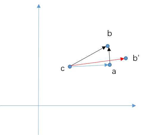
a. 计算每个slice的质心 c(其实可以理解为laser的位置,因为360°扫描);
b. 设置第一个点为参考点 a,因为排过序,所以第一个点应为与x轴角度最小的点;
c. 连接当前点 b(参考点的下一个点)和参考点 a,并计算它与x轴的夹角,按照夹角映射到直方图;
d. 计算该点的权重,即ab与bc的垂直程度,直方图元素即为权重的累加值。
理解:需要注意,当当前点和参考点超出一定距离时,需要重置参考点,因此当前点可以认为是参考点的临*点,处于一个邻域内;另外,需要格外注意的是,匹配过程中通常需要先将点云按照角分辨率和角度搜索窗口进行旋转,生成所有候选scan,然后在每个角度scan内匹配xyz窗口,而这里的这种匹配方法刚好对距离并不敏感,如对于同一个视角,c点距离ab的远*并不影响ab和bc的角度,同样不影响权重大小的计算,所以我觉得这种计算方法有一定道理,事实上它也是先通过这种方法筛选角度搜索窗口内的一些scan,然后在进行xyz*移的遍历,获得最优的*移;
权重的计算思想,当ab和bc*乎垂直时,说明ab可能是一个垂直于激光扫描线束的*面,这时探测结果应该是比较准确的,相反,如果ab'如何过b‘c*乎*行时,说明扫描线束*乎*行与障碍物,这时可能探测误差较大(可能由传感器引起,也有可能是孔洞、玻璃等),因此权重应该降低。
看代码:
直方图匹配入口,将直方图进行旋转,然后计算两个直方图的余弦距离;(注意:这里仅仅进行了yaw方向的旋转,同时这里没考虑这种直方图的计算方法直接进行旋转是否能保持不变性。)
std::vector<float> RotationalScanMatcher::Match(
    const Eigen::VectorXf& histogram, const float initial_angle,
    const std::vector<float>& angles) const { // angles属于(-theta, theta)范围;
  std::vector<float> result;
  result.reserve(angles.size());
  for (const float angle : angles) {
    // 将直方图进行旋转
    const Eigen::VectorXf scan_histogram = RotateHistogram(histogram, initial_angle + angle);

    //计算两个直方图的相似程度,余弦距离;
    result.push_back(MatchHistograms(*histogram_, scan_histogram));
  }
  return result;
}
// Rotates the given 'histogram' by the given 'angle'. This might lead to
// rotations of a fractional bucket which is handled by linearly interpolating.
Eigen::VectorXf RotationalScanMatcher::RotateHistogram(
    const Eigen::VectorXf& histogram, const float angle) {

  const float rotate_by_buckets = -angle * histogram.size() / M_PI;

  int full_buckets = common::RoundToInt(rotate_by_buckets - 0.5f);  //本来是四舍五入取整,减去0.5变成向下取整;注意是负数;
  const float fraction = rotate_by_buckets - full_buckets;  //总是一个小于1大于0的数;

  while (full_buckets < 0) {
    full_buckets += histogram.size();
  }

  Eigen::VectorXf rotated_histogram_0 = Eigen::VectorXf::Zero(histogram.size());
  Eigen::VectorXf rotated_histogram_1 = Eigen::VectorXf::Zero(histogram.size());
  for (int i = 0; i != histogram.size(); ++i) {
    rotated_histogram_0[i] = histogram[(i + full_buckets) % histogram.size()];
    rotated_histogram_1[i] = histogram[(i + 1 + full_buckets) % histogram.size()];
  }

  //貌似是一种计算插值的方法?
  return fraction * rotated_histogram_1 +
         (1.f - fraction) * rotated_histogram_0;
}
//计算两个直方图的余弦距离,即相似程度;
float MatchHistograms(const Eigen::VectorXf& submap_histogram,
                      const Eigen::VectorXf& scan_histogram) {
  // We compute the dot product of normalized histograms as a measure of
  // similarity.
  const float scan_histogram_norm = scan_histogram.norm();
  const float submap_histogram_norm = submap_histogram.norm();
  const float normalization = scan_histogram_norm * submap_histogram_norm;
  if (normalization < 1e-3f) {
    return 1.f;
  }
  return submap_histogram.dot(scan_histogram) / normalization;
}
直方图的计算过程:
计算直方图,将点云进行切片处理:
Eigen::VectorXf RotationalScanMatcher::ComputeHistogram(
    const sensor::PointCloud& point_cloud, const int histogram_size) {

  Eigen::VectorXf histogram = Eigen::VectorXf::Zero(histogram_size);

  std::map<int, sensor::PointCloud> slices;
  for (const sensor::RangefinderPoint& point : point_cloud) {

    // 将点云的z值放大5倍,然后四舍五入取整,将点云分割成为一些slices,每个slices中存放原始点集;
    slices[common::RoundToInt(point.position.z() / kSliceHeight)].push_back(point);

  }

  for (const auto& slice : slices) {
    AddPointCloudSliceToHistogram(SortSlice(slice.second), &histogram);
  }
  return histogram;
}
将slice中的点进行排序处理:即按照沿x轴的角度进行排序
// A function to sort the points in each slice by angle around the centroid.
// This is because the returns from different rangefinders are interleaved in
// the data.
sensor::PointCloud SortSlice(const sensor::PointCloud& slice) {

  struct SortableAnglePointPair {
    bool operator<(const SortableAnglePointPair& rhs) const {
      return angle < rhs.angle;
    }

    float angle;
    sensor::RangefinderPoint point;
  };

  //计算slice中点云的均值;
  const Eigen::Vector3f centroid = ComputeCentroid(slice);

  std::vector<SortableAnglePointPair> by_angle;
  by_angle.reserve(slice.size());

  for (const sensor::RangefinderPoint& point : slice) {

    const Eigen::Vector2f delta = (point.position - centroid).head<2>();  //提取该点距离中心点的前两维(x,y);
    // 确保这个点距离中心点足够远?
    if (delta.norm() < kMinDistance) {
      continue;
    }

    //atan2(delta)是一个在xoy*面内的角度值,具体的就是delta向量和x轴的角度;
    by_angle.push_back(SortableAnglePointPair{common::atan2(delta), point});
  }
  //将该slice中的点按照距离中点的在xoy*面内的角度值排序;
  std::sort(by_angle.begin(), by_angle.end());

  sensor::PointCloud result;
  //然后把排序好的结果中的point取出;
  for (const auto& pair : by_angle) {
    result.push_back(pair.point);
  }
  return result;
}
将slice中的点云映射到直方图中:
void AddPointCloudSliceToHistogram(const sensor::PointCloud& slice,
                                   Eigen::VectorXf* const histogram) {
  if (slice.empty()) {
    return;
  }
  // We compute the angle of the ray from a point to the centroid of the whole
  // point cloud. If it is orthogonal to the angle we compute between points, we
  // will add the angle between points to the histogram with the maximum weight.
  // This is to reject, e.g., the angles observed on the ceiling and floor.

  const Eigen::Vector3f centroid = ComputeCentroid(slice);  //又要计算一次中心点坐标;

  Eigen::Vector3f last_point_position = slice.front().position; //返回第一个元素的坐标;

  for (const sensor::RangefinderPoint& point : slice) {

    const Eigen::Vector2f delta = (point.position - last_point_position).head<2>(); //这是和参考点在xoy*面内的向量;

    const Eigen::Vector2f direction = (point.position - centroid).head<2>();  //这是和

    //第一个点,distance = 0,所以跳过;
    //确保前后两个点之间,以及当前点和中心点之间的距离都大于阈值;
    const float distance = delta.norm();
    if (distance < kMinDistance || direction.norm() < kMinDistance) {
      continue;
    }
    //如果距离太大,则重置参考点;所有点的都按照角度排过序;
    if (distance > kMaxDistance) {
      last_point_position = point.position;
      continue;
    }
    const float angle = common::atan2(delta); // 这是当前点和参考点之间的连线和x轴所成的夹角;

    //如果两个向量垂直,dot=0,如果两个向量*行,dot=1,这表示的是当前点和参考点之间,以及当前点和中心点之间向量的点积值;
    //所以,如果两个向量垂直,value值越大,两个向量越接**行,value值越小;
    const float value = std::max(0.f, 1.f - std::abs(delta.normalized().dot(direction.normalized())));

    // 按照angle将value值累加在histogram中;
    AddValueToHistogram(angle, value, histogram);
  }
}
直方图权重的计算方法:
void AddValueToHistogram(float angle, const float value,
                         Eigen::VectorXf* histogram) {
  // Map the angle to [0, pi), i.e. a vector and its inverse are considered to
  // represent the same angle.
  while (angle > static_cast<float>(M_PI)) {
    angle -= static_cast<float>(M_PI);
  }
  while (angle < 0.f) {
    angle += static_cast<float>(M_PI);
  }

  const float zero_to_one = angle / static_cast<float>(M_PI);

  const int bucket = common::Clamp<int>(  // 确保bucket一定在[0,size - 1]之间;
      common::RoundToInt(histogram->size() * zero_to_one - 0.5f), 0,
      histogram->size() - 1);

  // 将【0,pi】的范围分割成了一定离散范围;当前点和参考点的向量与当前点和中心的向量,越垂直权重越大
  // 直方图的理解:相当于将所有的点云分了size个类别,分类的标准为当前点和参考点之间与x轴的夹角,这样每个点都能划分到
  // 一个类别中,它在该类别中的占比为当前点和参考点的的连线与当前点与质心点之间连线的同向行,越垂直值越大,因为越*行
  // 说明可能是外点或对同一个点的不同测量?
  (*histogram)(bucket) += value;
}
2.3、然后对生成的离散Scan进行xyz三个方向上的分枝定界寻优算法,完成匹配过程。注释代码按顺序放在最后。
3、ceres scan matcher
需要注意的是,在前端的SLAM定位过程中,cartographer3D并没有像2D那样先使用scan matching确定初值,然后进行ceres优化,而是直接使用IMU提供的角速度进行积分,获得一个旋转初值,用于优化姿态,而如果有里程计,会给出一个*移的初值,如果没有里程计,该初值为0。因此前端定位直接是ceres优化,该优化过程没有什么可说的,需要注意的是其优化过程中将*移和旋转分辨设定了权重,这也是调参过程中需要注意的地方:
  //存储一些权重参数,即优化时的信息矩阵;
  options.set_translation_weight(
      parameter_dictionary->GetDouble("translation_weight"));
  options.set_rotation_weight(
      parameter_dictionary->GetDouble("rotation_weight"));
  options.set_only_optimize_yaw(
      parameter_dictionary->GetBool("only_optimize_yaw"));
  //优化参数,包括最大迭代次数、线程、单调性等;
  *options.mutable_ceres_solver_options() =
      common::CreateCeresSolverOptionsProto(
          parameter_dictionary->GetDictionary("ceres_solver_options").get());
  return options;
}

CeresScanMatcher3D::CeresScanMatcher3D(
    const proto::CeresScanMatcherOptions3D& options)
    : options_(options),
      ceres_solver_options_(
          common::CreateCeresSolverOptions(options.ceres_solver_options())) {
  ceres_solver_options_.linear_solver_type = ceres::DENSE_QR;
}

void CeresScanMatcher3D::Match(
    const Eigen::Vector3d& target_translation,  //所求的目标变换;
    const transform::Rigid3d& initial_pose_estimate,    //由scan matching或其它传感器提供的初始值;
    const std::vector<PointCloudAndHybridGridPointers>&
        point_clouds_and_hybrid_grids,  //混合的概率网格;
    transform::Rigid3d* const pose_estimate,
    ceres::Solver::Summary* const summary) {

  //首先声明一个ceres最小二乘问题;
  ceres::Problem problem;

  optimization::CeresPose ceres_pose(
      initial_pose_estimate, nullptr /* translation_parameterization */,
      options_.only_optimize_yaw() ? std::unique_ptr<ceres::LocalParameterization>(
                absl::make_unique<ceres::AutoDiffLocalParameterization<YawOnlyQuaternionPlus, 4, 1>>())
          : std::unique_ptr<ceres::LocalParameterization>(
                absl::make_unique<ceres::QuaternionParameterization>()),
      &problem);

  CHECK_EQ(options_.occupied_space_weight_size(),
           point_clouds_and_hybrid_grids.size());   // 这里点云所在的混合概率网格只有两层吗?因为选项中权重设置只有两个参数哇!!!
                               // 而且第一个为低分辨率的权重,第二个为高分辨率的权重,因此第一个权重应该远小于第二个权重;

  // 这是概率网格的残差构造;
  for (size_t i = 0; i != point_clouds_and_hybrid_grids.size(); ++i) {
    CHECK_GT(options_.occupied_space_weight(i), 0.);

    const sensor::PointCloud& point_cloud =
        *point_clouds_and_hybrid_grids[i].first;

    const HybridGrid& hybrid_grid = *point_clouds_and_hybrid_grids[i].second;

    problem.AddResidualBlock(
        // 构建自动求导的代价函数,即点云关于旋转和*移的残差项;
        OccupiedSpaceCostFunction3D::CreateAutoDiffCostFunction(
            // weight1 / sqrt(size),这是残差的一个系数,因为残差需要进行*方,因此开根号可以理解;
            options_.occupied_space_weight(i) / std::sqrt(static_cast<double>(point_cloud.size())),
            point_cloud, hybrid_grid),

        nullptr /* loss function */, ceres_pose.translation(),  // loss function 为nullptr时,表示使用残差的*方项;
        ceres_pose.rotation()
        );
  }
  // *移单独构造了一个残差函数,并且一块进行优化
  CHECK_GT(options_.translation_weight(), 0.);
  problem.AddResidualBlock(
      TranslationDeltaCostFunctor3D::CreateAutoDiffCostFunction(
          options_.translation_weight(), target_translation),
      nullptr /* loss function */, ceres_pose.translation());
  // 单独给*移和旋转构造一个残差函数!
  CHECK_GT(options_.rotation_weight(), 0.);
  problem.AddResidualBlock(
      RotationDeltaCostFunctor3D::CreateAutoDiffCostFunction(
          options_.rotation_weight(), initial_pose_estimate.rotation()),
      nullptr /* loss function */, ceres_pose.rotation());
  // 求解该问题;
  ceres::Solve(ceres_solver_options_, &problem, summary);

  *pose_estimate = ceres_pose.ToRigid();
}

 浙公网安备 33010602011771号