机器学习之Artificial Neural Networks

人类通过模仿自然界中的生物，已经发明了很多东西，比如飞机，就是模仿鸟翼，但最终，这些东西会和原来的东西有些许差异，artificial neural networks (ANNs)就是模仿动物大脑的神经网络。

ANNs是Deep Learning的基本组成部分，它有很多用处：

ANNs are at the very core of Deep Learning. They are versatile, powerful, and scala‐ ble, making them ideal to tackle large and highly complex Machine Learning tasks, such as classifying billions of images (e.g., Google Images), powering speech recogni‐ tion services (e.g., Apple’s Siri), recommending the best videos to watch to hundreds of millions of users every day (e.g., YouTube), or learning to beat the world champion at the game of Go by examining millions of past games and then playing against itself (DeepMind’s AlphaGo).

From Biological to Artificial Neurons

ANNs已经有很悠久的历史了，我们不谈历史，到目前为止，ANNs又重新焕发青春，主要有下边几个理由：

现在有大量高质量的数据来训练神经网络，并且ANNs更适宜大且复杂的问题
物理计算能力的巨大提升，为训练大型神经网络提供了基础，比如强大的GPU
训练算法有了一定的改进，性能得到很大提升
ANNs的理论局限性已经在实践中被证明是良性的，通过大量的实验，ANNs都体现了良好的效果，最大限度的接近全局最优解
资金流向ANNs，这同样极大刺激了它的发展

Biological Neurons

ANNs主要是模仿生物神经元，我们先简单了解一下生物神经元的组成：

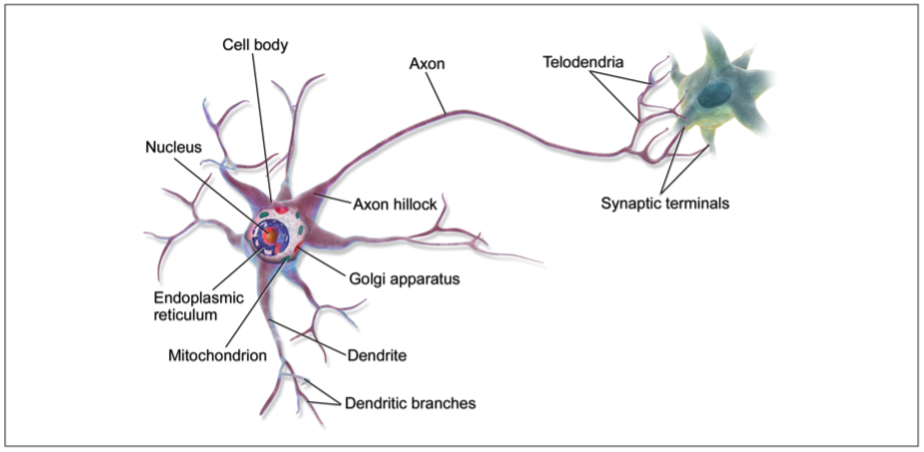
神经元由细胞体，树突，轴突和神经末梢组成：

细胞体的作用是处理树突传过来的各种信息，在ANNs中它就好比激活函数，用于决定当前神经元的输出
树突用于连接其他的神经元，在ANNs中它就像每个神经元和输入的连接
轴突是神经元的输出

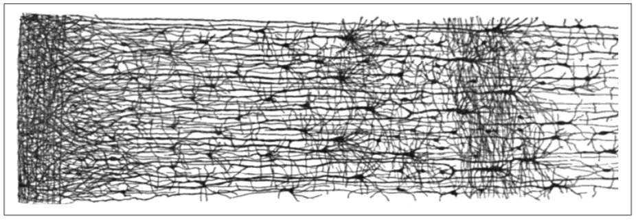
生物系统的神经元网络：

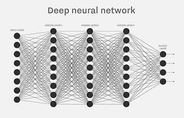
深度神经网络：

Logical Computations with Neurons

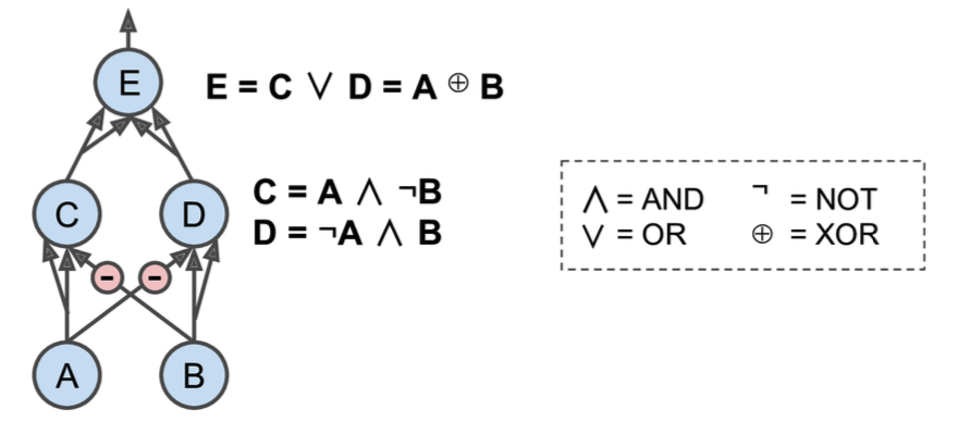
如果我们把神经元的输入和输出都设定为二进制（开或者关），我们能够利用ANNs实现一些逻辑运算，下边就是一个示例：

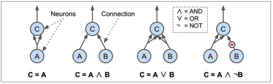
最左边的是一个identity函数，A的状态直接传递给C
第一个实现了逻辑AND，只有当A和B都激活的时候，C才被激活
第三个实现了逻辑OR， A或B任何一个被激活，C都会激活
第四个，只有A激活且B不激活的情况下，才能激活C

The Perceptron

Perceptron是ANNs架构的最简单的一种，它的神经元成为linear threshold unit (LTU)，我们后续都使用LTU这个名称，它的输入和输出都是数值类型，先看一张示意图：

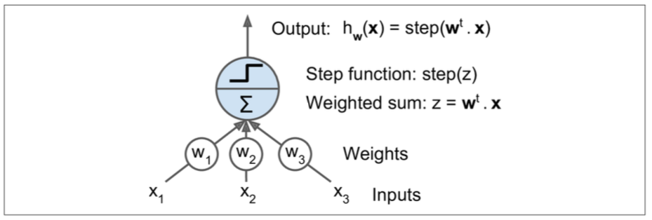
每个输入值都通过一个w(权值)和神经元链接，这时候神经元就是上边提到的LTU，LTU通过下边的公式计算输入的值：

\[z = w_1x_1 + w_2x_2 + \cdots + w_nx_n = \vec{w}^T \cdot \vec{x} \]

求和结束后，使用一个step function来再次计算要输出的值，公式如下：

\[h_w(\vec{x}) = step(z) = step(\vec{w}^T \cdot \vec{x}) \]

一般通用的step function有两个：

\[heaviside(z) = \begin{cases} 0 & \text{if $z < 0$} \\ 1 & \text{if $z \geq 0$} \end{cases} \]

\[sgn(z) = \begin{cases} -1 & \text{if $z < 0$} \\ 0 & \text{if $z = 0$} \\ 1 & \text{if $z > 0$} \end{cases} \]

看上图可知，一个单独的LTU可以做线性二进制分类，原理是，它对输入数据求和后，在根据一个threshold做判断，然后再输出类别。

Perceptron可以说是由单层的LTUs组成，我们已经知道LTUs是一个神经单元，如果把多个LTUs放到一层，作为输出层，再增加一个输入层，就构成了感知机。在输入层还需要增加一个偏置。如下图所示：

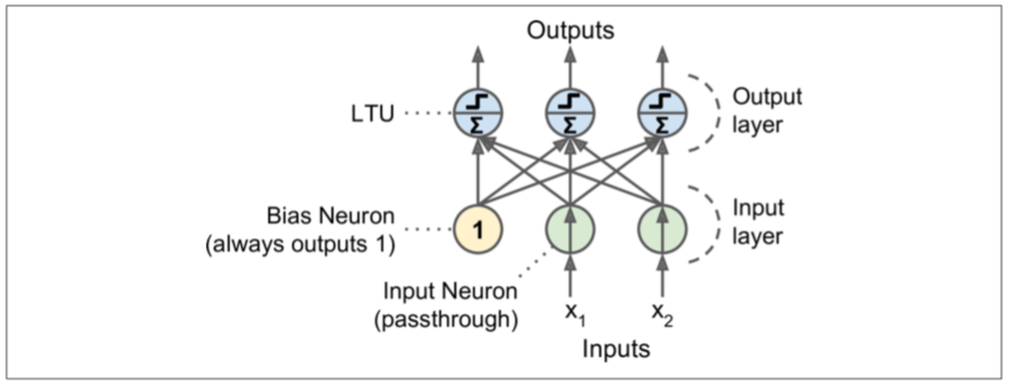
那么感知机是如何训练的呢？由上图可知，训练感知机就是获取这些链接中的权值w，自然地，如果某个LTU的预测值和实际值差别越大，w更新的步子就越大，因此，得出下边的公式：

\[w_{i,j}^{(next \ step)} = w_{i,j} + \eta(\hat{y_j} - y_j)x_i \]

$w_{i, j}$是第i个输入神经元和第j个输出神经元的权值
$x_i$是当前训练实例的第i个输入值
$\hat{y_j}$是当前训练实例的第j个神经元的输出值
$y_j$是当前训练实例的第j个神经元的实际值
$\eta$是学习率

由于每一个输出神经元的决策边界是线性的，所有感知机不能处理复杂的学习模式，比如逻辑回归分类。如果训练集是线性可分的，它是可以实现的。

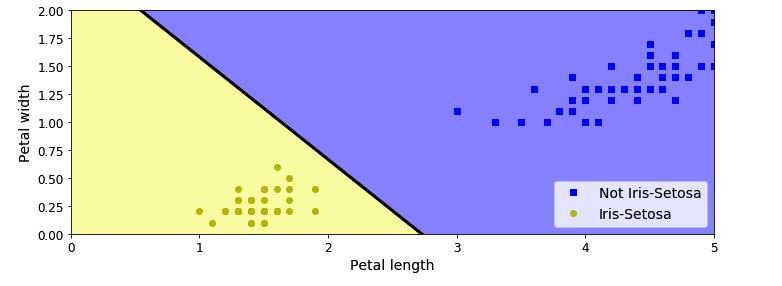
我们用代码实现一个iris分类的例子：

import numpy as np
from sklearn.datasets import load_iris
from sklearn.linear_model import Perceptron

iris = load_iris()
X = iris.data[:, (2, 3)]  # petal length, petal width
y = (iris.target == 0).astype(np.int)

per_clf = Perceptron(max_iter=100, tol=-np.infty, random_state=42)
per_clf.fit(X, y)

y_pred = per_clf.predict([[2, 0.5]])

"""
array([1])
"""

其实，感知机算法和随机梯度下降算法很相似，实际上Scikit-Learn的Perceptron类等同于使用SGDClassifier类，设置loss="perceptron" learning_rate="constant" eta=1 penalty=None。

相对于逻辑回归分类，感知机的缺点是它并不输出概率。它的预测只能根据一个hard threshold。这也是为什么选择逻辑回归分类的原因。

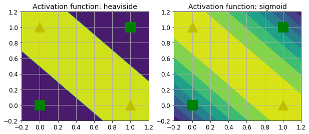
如果把感知机拓展到多层结构，就能够实现一些其他的功能，比如，实现XOR逻辑：

def heaviside(z):
    return (z >= 0).astype(z.dtype)

def mlp_xor(x1, x2, activation=heaviside):
    return activation(-activation(x1 + x2 - 1.5) + activation(x1 + x2 - 0.5) - 0.5)

上边的代码是按照下图设计的：

上边的代码中，使用的是heaviside激活函数，也可以使用其他激活函数，比如sigmoid，他们的决策边界对比如下：

Multi-Layer Perceptron and Backpropagation

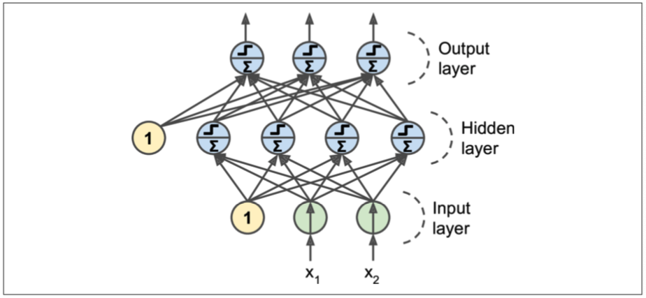
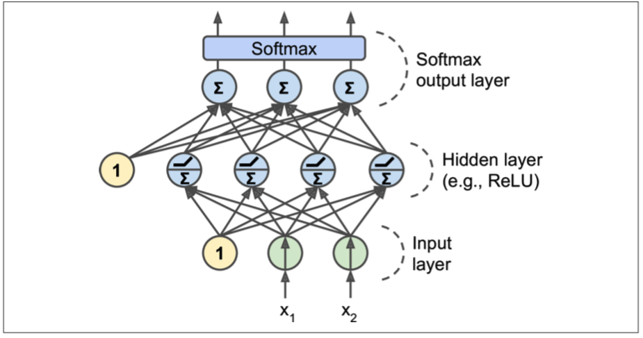
一个MLP由一个输入层，一层或多层LTUs（隐藏层）和一个输出层组成。除了输出层之外，其他的层都包含一个偏置。当一个ANN包含2个隐藏层时，成为deep neural network（DNN）。

下图是一个隐藏层的MLP：

对于MLP，在一开始，比较困难的是如何训练它，目前采用的算法是backpropagation，逆向传播算法。在介绍这个之前，我们先简单介绍一下TensorFlow的reverse-mode autodiff。

在TensorFlow中，首先正向的计算出各个node的值，然后利用链式法则，逆向的对每个node进行求导，用一张图就能很轻易的表示这个过程：

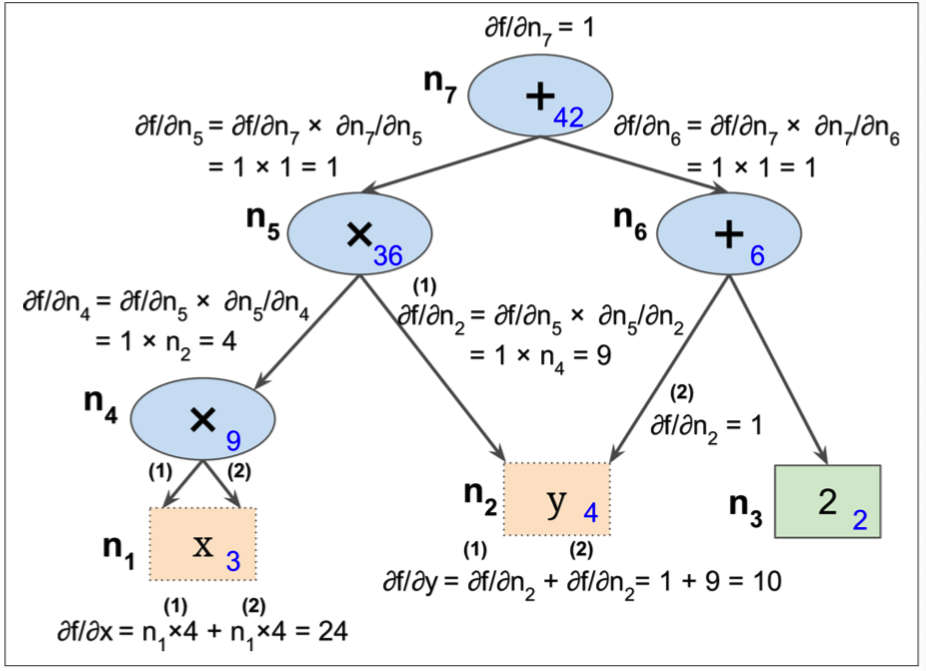
这其中有一个细节，以n5来举例，

\[\partial{n_7}/\partial{n_5} \]

这个是如何计算的呢？由于$n_7 = n_5 + n_6$，所以在计算$\partial{n_7}/\partial{n_5}$的偏导数的时候，得到的偏导数为1，下边的原理都是这样。整个偏导数的计算过程需要对图做两次遍历，首先正向求出每个node的值，然后反向遍历求各个node的偏导数。

我们在训练该算法中，最核心的问题是修正W，那么上边计算出来的偏导数就用上了，看下边这个图，它显示了逆向传播算法的基本原理和过程：

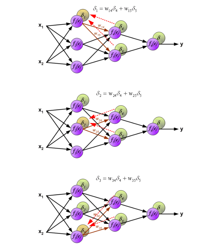
在上图中，首先正向的先计算出最后的误差$\delta$,然后利用node间链接的w计算出前一层各个node的$\delta$。这样我们就能够获得每个node的误差$\delta$。

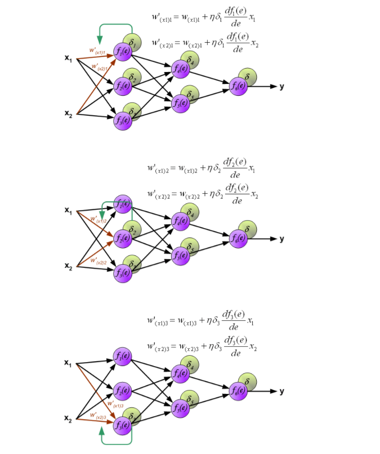
从上图可以很简单的看出，使用该node的梯度和误差，就可以计算出修正后的w。这其中，用到的激活函数，最常用的有下边三个：

logistic function $\sigma(z)=1/(1 + e^{-z})$
hyperbolic tangent function $tanh(z) = 2\sigma(2z) - 1$
ReLU function $Relu(z) = max(0, z)$

通过图表对比下他们的函数图形和导数图形：

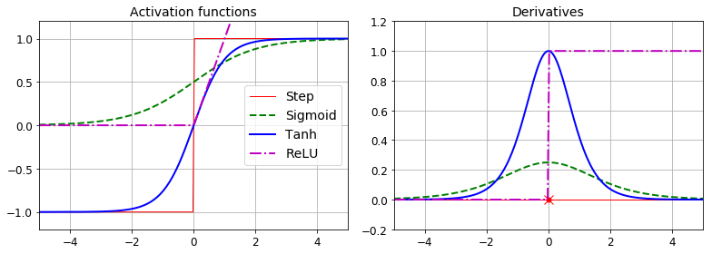
MLP经常被用来分类，它的输出层可以分别对应多个类别，因此我们需要对输出层的神经元的激活函数做一些特殊的处理，如果是分类任务，我们可以去掉输出层的激活函数，然后为它增加额外的softmax function。用来获取一些自定义的策略，比如控制threshold或者概率等等。

Training an MLP with TensorFlow’s High-Level API

如果使用TensorFlow的高层api来实现DNN，非常简单，我们看下代码实现：

获取数据：

import tensorflow as tf


(X_train, y_train), (X_test, y_test) = tf.keras.datasets.mnist.load_data()
X_train = X_train.astype(np.float32).reshape(-1, 28 * 28) / 255.0
X_test = X_test.astype(np.float32).reshape(-1, 28 * 28) / 255.0
y_train = y_train.astype(np.int32)
y_test = y_test.astype(np.int32)
X_valid, X_train = X_train[:5000], X_train[5000:]
y_valid, y_train = y_train[:5000], y_train[5000:]

核心代码,训练模型：

feature_cols = [tf.feature_column.numeric_column("X", shape=[28 * 28])]
dnn_clf = tf.estimator.DNNClassifier(hidden_units=[300, 100], n_classes=10, feature_columns=feature_cols)

input_fn = tf.estimator.inputs.numpy_input_fn(x={"X": X_train}, y=y_train, num_epochs=40, batch_size=50, shuffle=True)
dnn_clf.train(input_fn=input_fn)

TensorFlow提供了评估函数：

valid_input_fn = tf.estimator.inputs.numpy_input_fn(x={"X": X_valid}, y=y_valid, shuffle=False)
eval_results = dnn_clf.evaluate(input_fn=valid_input_fn)

"""
{'accuracy': 0.982,
 'average_loss': 0.09565534,
 'loss': 11.956917,
 'global_step': 44000}
"""

评估测试集：

test_input_fn = tf.estimator.inputs.numpy_input_fn(x={"X": X_test}, y=y_test, shuffle=False)
y_pred_iter = dnn_clf.predict(input_fn=test_input_fn)
y_pred = list(y_pred_iter)
y_pred[0]

"""
{'logits': array([ -7.4078193,   2.8550382,   1.8491653,   6.945245 ,  -5.996856 ,
         -0.6053193, -10.372234 ,  22.27766  ,  -4.490141 ,   2.99006  ],
       dtype=float32),
 'probabilities': array([1.2816213e-13, 3.6716565e-09, 1.3428177e-09, 2.1938979e-07,
        5.2545213e-13, 1.1535802e-10, 6.6119684e-15, 9.9999976e-01,
        2.3707813e-12, 4.2024433e-09], dtype=float32),
 'class_ids': array([7]),
 'classes': array([b'7'], dtype=object),
 'all_class_ids': array([0, 1, 2, 3, 4, 5, 6, 7, 8, 9], dtype=int32),
 'all_classes': array([b'0', b'1', b'2', b'3', b'4', b'5', b'6', b'7', b'8', b'9'],
       dtype=object)}
"""

从上边最后一个代码块可以看出，它输出了每个类别的概率值。

Training a DNN Using Plain TensorFlow

如果相对神经网络有更灵活的控制，我们就需要使用TensorFlow的底层api。

Construction Phase

首先，我们定义一些属性，包括输入层的维度，各个隐藏层包含的神经元个数，输出层的神经元个数，我们用X和y表示输入的数据目标值：

n_inputs = 28 * 28
n_hidden1 = 300
n_hidden2 = 100
n_outputs = 10

reset_graph()

X = tf.placeholder(tf.float32, shape=(None, n_inputs), name="X")
y = tf.placeholder(tf.int32, shape=(None), name="y")

接下来，我们需要写一个函数来描述神经网络的某一层，可能是隐藏层，也可能是输出层，他们大致上是相似的，区别只是是否包含激活函数，函数如下：

def neuron_layer(X, n_neurons, name, activation=None):
    with tf.name_scope(name):
        n_inputs = int(X.get_shape()[1])
        stddev = 2 / np.sqrt(n_inputs)
        init = tf.truncated_normal((n_inputs, n_neurons), stddev=stddev)
        W = tf.Variable(init, name="kernel")
        b = tf.Variable(tf.zeros([n_neurons]), name="bias")
        Z = tf.matmul(X, W) + b
        if activation is not None:
            return activation(Z)
        else:
            return Z

我们对上边函数做一个详细的说明：

通过name给每一层加一个名称域，这么做的好处是在用TensorBoard看图的结构时，更加清晰
n_inputs用户计算该层输入数据的特征的个数
第三部主要用于计算该层与上一层的权值矩阵,(n_inputs, n_neurons)保存着上一层中每个神经元与该层链接的权值，权值通过随机的方式产生，符合高斯正态分布
为该层的每个神经元添加一个偏置
计算该层的输出值，这里是一个输出矩阵，每一行保存着该层的神经元的值
如果指定了激活函数，则调用激活函数计算结果，否则直接输出结果

基于上边的函数，定义神经网络模型：

with tf.name_scope("dnn"):
    hidden1 = neuron_layer(X, n_hidden1, name="hidden1", activation=tf.nn.relu)
    hidden2 = neuron_layer(hidden1, n_hidden2, name="hidden2", activation=tf.nn.relu)
    logits = neuron_layer(hidden2, n_outputs, name="outputs")

接下来我们需要定义代价函数，我们使用交叉熵来计算误差：

with tf.name_scope("loss"):
    xentropy = tf.nn.sparse_softmax_cross_entropy_with_logits(labels=y, logits=logits)
    loss = tf.reduce_mean(xentropy, name="loss")

定义训练模型：

learning_rate = 0.01

with tf.name_scope("train"):
    optimizer = tf.train.GradientDescentOptimizer(learning_rate)
    training_op = optimizer.minimize(loss)

定义评估模块：

with tf.name_scope("eval"):
    correct = tf.nn.in_top_k(logits, y, 1)
    accuracy = tf.reduce_mean(tf.cast(correct, tf.float32))

初始化变量：

init = tf.global_variables_initializer()
saver = tf.train.Saver()

Execution Phase

我们再改算法中需要使用小批次梯度下降算法，因此我们先定义一个随机产生批次函数：

n_epochs = 40
batch_size = 50

def shuffle_batch(X, y, batch_size):
    rnd_idx = np.random.permutation(len(X))
    n_batches = len(X) // batch_size
    for batch_idx in np.array_split(rnd_idx, n_batches):
        X_batch, y_batch = X[batch_idx], y[batch_idx]
        yield X_batch, y_batch

执行代码：

with tf.Session() as sess:
    init.run()
    for epoch in range(n_epochs):
        for X_batch, y_batch in shuffle_batch(X_train, y_train, batch_size):
            sess.run(training_op, feed_dict={X: X_batch, y: y_batch})
        acc_batch = accuracy.eval(feed_dict={X: X_batch, y: y_batch})
        acc_val = accuracy.eval(feed_dict={X: X_valid, y: y_valid})
        print(epoch, "Batch accuracy:", acc_batch, "Val accuracy:", acc_val)

    save_path = saver.save(sess, "./my_model_final.ckpt")

训练过程输出如下：

0 Batch accuracy: 0.9 Val accuracy: 0.9146
1 Batch accuracy: 0.92 Val accuracy: 0.936
2 Batch accuracy: 0.96 Val accuracy: 0.945
...
37 Batch accuracy: 1.0 Val accuracy: 0.9776
38 Batch accuracy: 1.0 Val accuracy: 0.9792
39 Batch accuracy: 1.0 Val accuracy: 0.9776

Using the Neural Network

with tf.Session() as sess:
    saver.restore(sess, "./my_model_final.ckpt") # or better, use save_path
    X_new_scaled = X_test[:20]
    Z = logits.eval(feed_dict={X: X_new_scaled})
    y_pred = np.argmax(Z, axis=1)

print("Predicted classes:", y_pred)
print("Actual classes:   ", y_test[:20])

"""
Predicted classes: [7 2 1 0 4 1 4 9 5 9 0 6 9 0 1 5 9 7 3 4]
Actual classes:    [7 2 1 0 4 1 4 9 5 9 0 6 9 0 1 5 9 7 3 4]
"""

上边代码中的neuron_layer是我们自定义的创建神经网络层的函数，在开发中，也可以使用TensorFlow提供的dense()函数来替代，效果一样, 上边代码只改动很少的一部分：

with tf.name_scope("dnn"):
    hidden1 = tf.layers.dense(X, n_hidden1, name="hidden1", activation=tf.nn.relu)
    hidden2 = tf.layers.dense(hidden1, n_hidden2, name="hidden2", activation=tf.nn.relu)
    logits = tf.layers.dense(hidden2, n_outputs, name="outputs")

Fine-Tuning Neural Network Hyperparameters

神经网络的灵活性同样也是它最主要的缺点，因为有太多的参数可以调整，比方说，网络拓扑，层数，每一层神经元的个数，每一层的激活函数，权值初始化等等很多参数，那么如何来获取最优的参数呢？

当然，我们可以使用grid search方法，但这种方法需要花费大量的时间，并且只能计算出一部分参数。用randomized search方法是一个很不错的方法。另外一个工具是Oscar,它提供更加负责的算法来快速计算最优参数。

Number of Hidden Layers

对于大多数问题，在最初，只需要定义一个隐藏层就能获得不错的效果。当然如果问题比较复杂，可能该层需要非常多的神经元，这种情况，把神经元个数分散到多层，会取得更多好的性能。

神经网络之所以是多层架构，原因是这种多层架构有很多好处，首先现实中的数据，往往是多层架构

我们以识别手写数字为例,

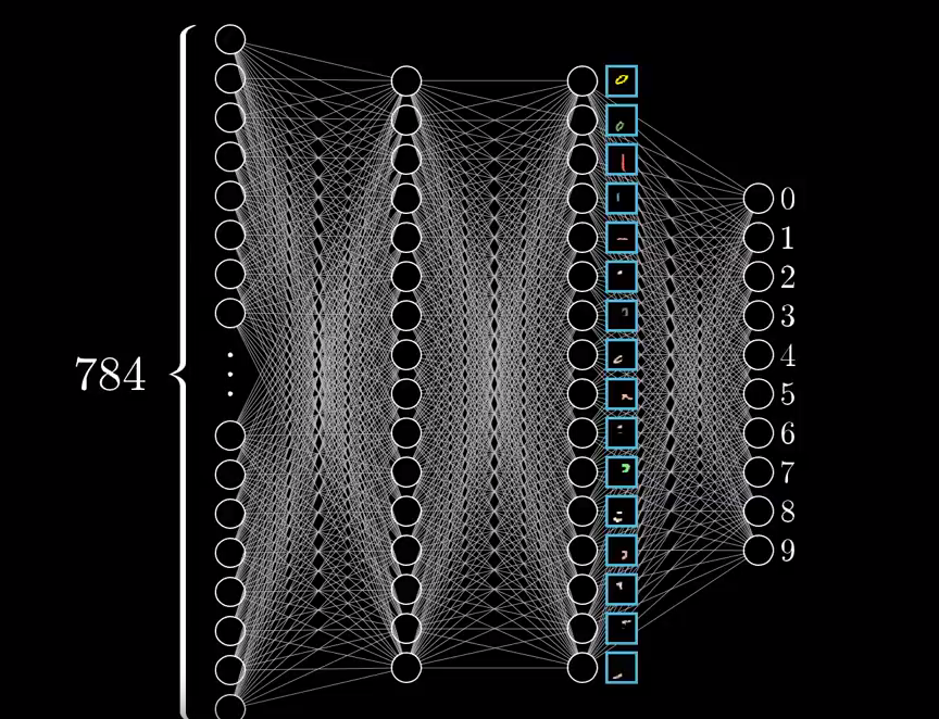
在神经网络的第一个隐藏层，通过映射，可以把数字隐身成很简单的图形结构，比如说一横，一竖等等，在第二个隐藏层，用上一层的简单结构组和成更复杂的图形，比如一个圈，一个更长的竖杠，越往后边的层次，能够描述的图形越复杂。

方向 ,线段 -> 矩形，圆 -> 更复杂的图形

这种分层架构让神经网络能够轻易适配到新的数据集上，可以把某个神经网络作为另一个神经网络的隐藏层，这大大节省了训练时间。

总之，对于大多数的问题，只需要一到两层的隐藏层就能够获得满意的效果，对于更复杂的问题，可以逐渐增加隐藏层的数量，直到训练集出现过拟为止。那种更复杂的问题，则需要更多的隐藏层和训练数据。

Number of Neurons per Hidden Layer

输入层和输出层的个数需要根据实际问题来定义，至于隐藏层中神经元的个数，一般来说，可以遵循漏斗模式，也就是说神经元的数目随着层次的递增原来越少，整体呈现漏斗的样式。原因就是我们上边说的，越往后，描述的结构就越复杂，相应的数量也就越少。

但是，目前一般采取的常用做法是，为每个隐藏层定义某个相同的数量，然后再计算最优参数时，把该个数作为一个可优化的参数, 能够大大简化计算过程。

一个最简单的方法是，在选择模型时，使用的层数和每层的个数要超过我们需要的个数，然后再使用early stopping来停止算法。

Activation Functions

激活函数涉及了梯度是否饱和的问题，通常情况下，使用ReLU就可以了。对于分类任务，输出层一般使用softmax激活函数，对于逻辑任务，则输出层不适用激活函数。

Exercises

1. Draw an ANN using the original artificial neurons (like the ones in Figure 10-3) that computes A ⊕ B (where ⊕ represents the XOR operation). Hint: A ⊕ B = (A∧ ¬ B) ∨ (¬ A ∧ B).

2. Why is it generally preferable to use a Logistic Regression classifier rather than a classical Perceptron (i.e., a single layer of linear threshold units trained using the Perceptron training algorithm)? How can you tweak a Perceptron to make it equivalent to a Logistic Regression classifier?

A classical Perceptron will converge only if the dataset is linearly separable, and it won’t be able to estimate class probabilities. In contrast, a Logistic Regression classifier will converge to a good solution even if the dataset is not linearly sepa‐ rable, and it will output class probabilities. If you change the Perceptron’s activa‐ tion function to the logistic activation function (or the softmax activation function if there are multiple neurons), and if you train it using Gradient Descent (or some other optimization algorithm minimizing the cost function, typically cross entropy), then it becomes equivalent to a Logistic Regression classifier.

3. Why was the logistic activation function a key ingredient in training the first MLPs?

The logistic activation function was a key ingredient in training the first MLPs because its derivative is always nonzero, so Gradient Descent can always roll down the slope. When the activation function is a step function, Gradient Descent cannot move, as there is no slope at all.

4. Name three popular activation functions. Can you draw them?

The step function, the logistic function, the hyperbolic tangent, the rectified lin‐ ear unit (see Figure 10-8). See Chapter 11 for other examples, such as ELU and variants of the ReLU.

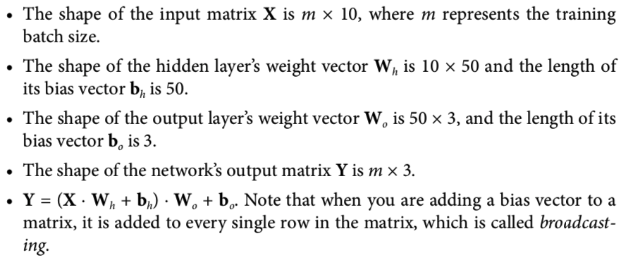
5. Suppose you have an MLP composed of one input layer with 10 passthrough neurons, followed by one hidden layer with 50 artificial neurons, and finally one output layer with 3 artificial neurons. All artificial neurons use the ReLU activa‐ tion function.

What is the shape of the input matrix X?
What about the shape of the hidden layer’s weight vector $W_h$, and the shape of

its bias vector $b_h$?
What is the shape of the output layer’s weight vector $W_o$, and its bias vector $b_o$?
What is the shape of the network’s output matrix Y?
Write the equation that computes the network’s output matrix Y as a function of X, $W_h$, $b_h$, $W_o$ and $b_o$.

6. How many neurons do you need in the output layer if you want to classify email into spam or ham? What activation function should you use in the output layer? If instead you want to tackle MNIST, how many neurons do you need in the out‐ put layer, using what activation function? Answer the same questions for getting your network to predict housing prices as in Chapter 2.

To classify email into spam or ham, you just need one neuron in the output layer of a neural network—for example, indicating the probability that the email is spam. You would typically use the logistic activation function in the output layer when estimating a probability. If instead you want to tackle MNIST, you need 10 neurons in the output layer, and you must replace the logistic function with the softmax activation function, which can handle multiple classes, outputting one probability per class. Now, if you want your neural network to predict housing prices like in Chapter 2, then you need one output neuron, using no activation function at all in the output layer.4

7. What is backpropagation and how does it work? What is the difference between backpropagation and reverse-mode autodiff?

Backpropagation is a technique used to train artificial neural networks. It first computes the gradients of the cost function with regards to every model parame‐ ter (all the weights and biases), and then it performs a Gradient Descent step using these gradients. This backpropagation step is typically performed thou‐ sands or millions of times, using many training batches, until the model parame‐ ters converge to values that (hopefully) minimize the cost function. To compute the gradients, backpropagation uses reverse-mode autodiff (although it wasn’t called that when backpropagation was invented, and it has been reinvented sev‐ eral times). Reverse-mode autodiff performs a forward pass through a computa‐ tion graph, computing every node’s value for the current training batch, and then it performs a reverse pass, computing all the gradients at once (see Appendix Dfor more details). So what’s the difference? Well, backpropagation refers to the whole process of training an artificial neural network using multiple backpropa‐ gation steps, each of which computes gradients and uses them to perform a Gra‐ dient Descent step. In contrast, reverse-mode autodiff is a simply a technique to compute gradients efficiently, and it happens to be used by backpropagation.

8. Can you list all the hyperparameters you can tweak in an MLP? If the MLP over‐ fits the training data, how could you tweak these hyperparameters to try to solve the problem?

Here is a list of all the hyperparameters you can tweak in a basic MLP: the num‐ ber of hidden layers, the number of neurons in each hidden layer, and the activa‐ tion function used in each hidden layer and in the output layer.5 In general, the ReLU activation function (or one of its variants; see Chapter 11) is a good default for the hidden layers. For the output layer, in general you will want the logistic activation function for binary classification, the softmax activation function for multiclass classification, or no activation function for regression.

If the MLP overfits the training data, you can try reducing the number of hidden layers and reducing the number of neurons per hidden layer.

9. Train a deep MLP on the MNIST dataset and see if you can get over 98% preci‐ sion. Just like in the last exercise of Chapter 9, try adding all the bells and whistles (i.e., save checkpoints, restore the last checkpoint in case of an interruption, add summaries, plot learning curves using TensorBoard, and so on).

这一题需要注意的有两点，一个是如何保存模型的断点，另一个是如何early stopping，代码如下：

from datetime import datetime


reset_graph()

X = tf.placeholder(tf.float32, shape=(None, n_inputs), name="X")
y = tf.placeholder(tf.int32, shape=(None), name="y")
with tf.name_scope("dnn"):
    hidden1 = tf.layers.dense(X, n_hidden1, name="hidden1", activation=tf.nn.relu)
    hidden2 = tf.layers.dense(hidden1, n_hidden2, name="hidden2", activation=tf.nn.relu)
    logits = tf.layers.dense(hidden2, n_outputs, name="outputs")

with tf.name_scope("loss"):
    xentropy = tf.nn.sparse_softmax_cross_entropy_with_logits(labels=y, logits=logits)
    loss = tf.reduce_mean(xentropy, name="loss")
    loss_summary = tf.summary.scalar('log_loss', loss)
    
learning_rate = 0.01

with tf.name_scope("train"):
    optimizer = tf.train.GradientDescentOptimizer(learning_rate)
    training_op = optimizer.minimize(loss)
    
with tf.name_scope("eval"):
    correct = tf.nn.in_top_k(logits, y, 1)
    accuracy = tf.reduce_mean(tf.cast(correct, tf.float32))
    accuracy_summary = tf.summary.scalar('accuracy', accuracy)
    
init = tf.global_variables_initializer()
saver = tf.train.Saver()

def log_dir(prefix=""):
    now = datetime.utcnow().strftime("%Y%m%d%H%M%S")
    root_logdir = "tf_logs"
    if prefix:
        prefix += "_"
    name = prefix + "run_" + now
    return "{}/{}/".format(root_logdir, name)

logdir = log_dir("mnist_dnn")

file_writer = tf.summary.FileWriter(logdir, tf.get_default_graph())

m, n = X_train.shape
n_epochs = 10001
batch_size = 50
n_batches = int(np.ceil(m / batch_size))

checkpoint_path = "/tmp/my_deep_mnist_model.ckpt"
checkpoint_epoch_path = checkpoint_path + ".epoch"
fimal_model_path = './my_deep_mnist_model'

best_loss = np.infty
epochs_without_progress = 0
max_epochs_without_progress = 50

def shuffle_batch(X, y, batch_size):
    rnd_idx = np.random.permutation(len(X))
    n_batches = len(X) // batch_size
    for batch_idx in np.array_split(rnd_idx, n_batches):
        X_batch, y_batch = X[batch_idx], y[batch_idx]
        yield X_batch, y_batch
        
with tf.Session() as sess:
    if os.path.isfile(checkpoint_epoch_path):
        # if the checkpoint file exists, restore the model and load the epoch number
        with open(checkpoint_epoch_path, "rb") as f:
            start_epoch = int(f.read())
        print("Training was interrupter. Continuing at epoch", start_epoch)
        saver.restore(sess, checkpoint_path)
    else:
        start_epoch = 0
        sess.run(init)
        
    for epoch in range(start_epoch, n_epochs):
        for X_batch, y_batch in shuffle_batch(X_train, y_train, batch_size):
            sess.run(training_op, feed_dict={X: X_batch, y: y_batch})
        accuracy_val, loss_val, accuracy_summary_str, loss_summary_str = sess.run([accuracy, loss, accuracy_summary, loss_summary], 
                                                                                  feed_dict={X: X_valid, y: y_valid})
        file_writer.add_summary(accuracy_summary_str, epoch)
        file_writer.add_summary(loss_summary_str, epoch)
        if epoch % 5 == 0:
            print("Epoch:", epoch, "\tValidation accuracy: {:.3f}%".format(accuracy_val * 100), "\tLoss: {:.5f}".format(loss_val))
            saver.save(sess, checkpoint_path)
            
            with open(checkpoint_epoch_path, "wb") as f:
                f.write(b"%d" % (epoch + 1))
            if loss_val < best_loss: 
                saver.save(sess, fimal_model_path)
                best_loss = loss_val 
            else: 
                epochs_without_progress += 5
                if epochs_without_progress > max_epochs_without_progress:
                    print("Early stopping")
                    break

posted @ 2019-09-22 16:59 马在路上阅读(1082) 评论(0) 编辑收藏举报

会员力量，点亮园子希望

刷新页面返回顶部

马在路上

一直在学习,一直在进步,乐在其中