
机器学习之TensorFlow介绍
TensorFlow的概念很简单:使用python定义一个计算图,然后TensorFlow根据计算图生成高性能的c++代码。

如上图所示,使用图的方式实现了函数\(f(x,y)=x^2y+y+2\)的计算,在图中可以定义操作符和输入输出变量,基于此特性,TensorFlow能够实现分布式的计算,可以实现大量特征和实例的训练任务。

上图,显示了多个GPU计算的过程,TensorFlow有一下几个优点:
- 支持多平台,Windows, Linux,macOS,iOS,Android
- 提供了简单的python api
- 有大量的其他的基于TensorFlow的高一级的库
- 可扩展性
- 高性能的c++实现
- 提供了很多方便计算代价函数的节点,带有自动求导功能
- 提供了强大的可视化工具TensorBoard
- 提供了云计算能力
- 开发社区比较活跃
下边是,目前比较常见的深度学习开源库:
Creating Your First Graph and Running It in a Session
我们用TensorFlow来写代码实现\(f(x,y)=x^2y+y+2\)
import tensorflow as tf


reset_graph()

x = tf.Variable(3, name='x')
y = tf.Variable(4, name='y')
f = x * x * y + y + 2
值得注意的是,此时TensorFlow并没有真正的创建这些变量,只创建了这样一幅计算图,要想执行这个计算,需要调用下边的代码,TensorFlow会自动把计算调度到cup或gpu。
sess = tf.Session()
sess.run(x.initializer)
sess.run(y.initializer)
result = sess.run(f)
print(result)
sess.close()
也可以使用python中的with关键词,简化代码:
with tf.Session() as sess:
    x.initializer.run()
    y.initializer.run()
    result = f.eval()

"""
42
"""
在with代码块内,session被设置为了默认的,当调用x.initializer.run()就相当于调用了tf.get_default_session().run(x.initial izer),f.eval()就相当于调用了tf.get_default_session().run(f),这么做的目的是让程序更加易读。
有时候,整个图的参数可能会有多个,TensorFlow提供了初始化这些变量的快捷方法:
init = tf.global_variables_initializer()

with tf.Session() as sess:
    init.run()
    result1 = f.eval()
TensorFlow程序一般分为两个步骤:首先创建计算图,其次运行。
Managing Graphs
创建的任何节点默认的都会被添加到默认的图中,我们用代码验证下:
reset_graph()

x1 = tf.Variable(1)
x1.graph is tf.get_default_graph()

'''
True
'''
在一般情况下,这基本上没问题,但是如果需要处理多个图,我们更希望往不同的图中添加变量,要实现这个想法,需要在创建一个新的图后,使用with把它暂时赋值为默认的图。
graph = tf.Graph()
with graph.as_default():
    x2 = tf.Variable(2)
x2.graph is graph

'''
True
'''

x2.graph is tf.get_default_graph()

'''
False
'''
Lifecycle of a Node Value
当evaluate一个节点的时候,TensorFlow自动判断改节点的依赖节点,并先执行依赖节点。举个例子:
w = tf.constant(3)
x=w+2
y=x+5
z=x*3

with tf.Session() as sess:
  print(y.eval()) # 10
  print(z.eval()) # 15
当执行y.eval()这行代码的时候,TensorFlow自动判断出它依赖x,x又依赖w,因此它首先计算w,然后再计算x,再计算y,计算z同上,但是默认的,它会计算x和w两次。
All node values are dropped between graph runs, except variable values, which are maintained by the session across graph runs (queues and readers also maintain some state, as we will see in Chapter 12). A variable starts its life when its initializer is run, and it ends when the session is closed.
对于上边的代码,如果想x和w只执行一次,可以这么写:
with tf.Session() as sess:
	y_val, z_val = sess.run([y, z])
  	print(y_val) # 10
 	 	print(z_val) # 15
In single-process TensorFlow, multiple sessions do not share any state, even if they reuse the same graph (each session would have its own copy of every variable). In distributed TensorFlow (see Chap‐ ter 12), variable state is stored on the servers, not in the sessions, so multiple sessions can share the same variables.
Linear Regression with TensorFlow
TensorFlow operations简称为ops,能够接受任何数量的输入和任何数量的输出,比如加法和乘法操作符,他们可以接受2个输入,并产生一个输出,Constants和variables不需要输人,它输出一个值。如果输入和输出是多维数组,则成为“tensor(张量)”。
下边的代码使用TensorFlow实现了线性回归:
import numpy as np
from sklearn.datasets import fetch_california_housing


reset_graph()

housing = fetch_california_housing()
m, n = housing.data.shape
housing_data_plus_bias = np.c_[np.ones((m, 1)), housing.data]

X = tf.constant(housing_data_plus_bias, dtype=tf.float32, name='X')
y = tf.constant(housing.target.reshape(-1, 1), dtype=tf.float32, name='y')

XT = tf.transpose(X)

theta = tf.matmul(tf.matmul(tf.matrix_inverse(tf.matmul(XT, X)), XT), y)

with tf.Session() as sess:
    theta_value = theta.eval()

"""
array([[-3.68962631e+01],
       [ 4.36777472e-01],
       [ 9.44449380e-03],
       [-1.07348785e-01],
       [ 6.44962370e-01],
       [-3.94082872e-06],
       [-3.78797273e-03],
       [-4.20847952e-01],
       [-4.34020907e-01]], dtype=float32)
"""
我们用最原始的数学表达式编码如下:
X = housing_data_plus_bias
y = housing.target.reshape(-1, 1)
theta_numpy = np.linalg.inv(X.T.dot(X)).dot(X.T).dot(y)

print(theta_numpy)

"""
[[-3.69419202e+01]
 [ 4.36693293e-01]
 [ 9.43577803e-03]
 [-1.07322041e-01]
 [ 6.45065694e-01]
 [-3.97638942e-06]
 [-3.78654265e-03]
 [-4.21314378e-01]
 [-4.34513755e-01]]
"""
使用Scikit-Learn:
from sklearn.linear_model import LinearRegression
lin_reg = LinearRegression()
lin_reg.fit(housing.data, housing.target.reshape(-1, 1))

print(np.r_[lin_reg.intercept_.reshape(-1, 1), lin_reg.coef_.T])

"""
[[-3.69419202e+01]
 [ 4.36693293e-01]
 [ 9.43577803e-03]
 [-1.07322041e-01]
 [ 6.45065694e-01]
 [-3.97638942e-06]
 [-3.78654265e-03]
 [-4.21314378e-01]
 [-4.34513755e-01]]
"""
可以看出,结果都是一样的,TensorFlow的主要优点是它会自动把数据的计算放到GPU卡。
Implementing Gradient Descent
实现上一小节中的线性回归,也可以使用梯度下降算法,在这里,我们使用Batch Gradient Descent。在使用这个算法之前,一定要先对数据做正则化。
from sklearn.preprocessing import StandardScaler
scaler = StandardScaler()
scaled_housing_data = scaler.fit_transform(housing.data)
scaled_housing_data_plus_bias = np.c_[np.ones((m, 1)), scaled_housing_data]
Manually Computing the Gradients
我们首先采用手动计算梯度的方式编码,由于原理比较简单,这里只贴出代码:
reset_graph()

n_epochs = 1000
learning_rate = 0.01

X = tf.constant(scaled_housing_data_plus_bias, dtype=tf.float32, name="X")
y = tf.constant(housing.target.reshape(-1, 1), dtype=tf.float32, name="y")
theta = tf.Variable(tf.random_uniform([n + 1, 1], -1.0, 1.0, seed=42), name="theta")
y_pred = tf.matmul(X, theta, name="predictions")
error = y_pred - y
mse = tf.reduce_mean(tf.square(error), name="mse")
gradients = 2/m * tf.matmul(tf.transpose(X), error)
training_op = tf.assign(theta, theta - learning_rate * gradients)

init = tf.global_variables_initializer()

with tf.Session() as sess:
    sess.run(init)

    for epoch in range(n_epochs):
        if epoch % 100 == 0:
            print("Epoch", epoch, "MSE =", mse.eval())
        sess.run(training_op)

    best_theta = theta.eval()

"""

Epoch 0 MSE = 9.161542
Epoch 100 MSE = 0.7145004
Epoch 200 MSE = 0.56670487
Epoch 300 MSE = 0.5555718
Epoch 400 MSE = 0.5488112
Epoch 500 MSE = 0.5436363
Epoch 600 MSE = 0.5396291
Epoch 700 MSE = 0.5365092
Epoch 800 MSE = 0.53406775
Epoch 900 MSE = 0.5321473
"""

best_theta

"""
array([[ 2.0685523 ],
       [ 0.8874027 ],
       [ 0.14401656],
       [-0.34770882],
       [ 0.36178368],
       [ 0.00393811],
       [-0.04269556],
       [-0.6614529 ],
       [-0.6375279 ]], dtype=float32)
"""
可以明显的看出来,随着迭代的进行,MSE逐渐收敛。
Using autodiff
使用TensorFlow的tf.gradients()可以自动求导,代码变得更加简洁:
reset_graph()

n_epochs = 1000
learning_rate = 0.01

X = tf.constant(scaled_housing_data_plus_bias, dtype=tf.float32, name="X")
y = tf.constant(housing.target.reshape(-1, 1), dtype=tf.float32, name="y")
theta = tf.Variable(tf.random_uniform([n + 1, 1], -1.0, 1.0, seed=42), name="theta")
y_pred = tf.matmul(X, theta, name="predictions")
error = y_pred - y
mse = tf.reduce_mean(tf.square(error), name="mse")

gradients = tf.gradients(mse, [theta])[0]

training_op = tf.assign(theta, theta - learning_rate * gradients)

init = tf.global_variables_initializer()

with tf.Session() as sess:
    sess.run(init)

    for epoch in range(n_epochs):
        if epoch % 100 == 0:
            print("Epoch", epoch, "MSE =", mse.eval())
        sess.run(training_op)

    best_theta = theta.eval()

print("Best theta:")
print(best_theta)

"""
Epoch 0 MSE = 9.161542
Epoch 100 MSE = 0.71450037
Epoch 200 MSE = 0.56670487
Epoch 300 MSE = 0.5555718
Epoch 400 MSE = 0.54881126
Epoch 500 MSE = 0.5436363
Epoch 600 MSE = 0.53962916
Epoch 700 MSE = 0.5365092
Epoch 800 MSE = 0.53406775
Epoch 900 MSE = 0.5321473
Best theta:
[[ 2.0685523 ]
 [ 0.8874027 ]
 [ 0.14401656]
 [-0.3477088 ]
 [ 0.36178365]
 [ 0.00393811]
 [-0.04269556]
 [-0.66145283]
 [-0.6375278 ]]
"""
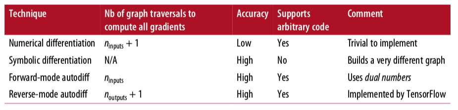
TensorFlow采用reverse-mode autodiff,这个模式比较使用于有大量输入和少量输出的情况。下图显示了其他模式:
Using an Optimizer
TensorFlow还提供了更方便的optimizer功能,Gradient Descent optimizer属于optimizer的一个特例,只需要改动很少的代码就能实现。
只需要把上边代码中的
gradients = tf.gradients(mse, [theta])[0]
training_op = tf.assign(theta, theta - learning_rate * gradients)
替换成下边的代码就可以了
optimizer = tf.train.GradientDescentOptimizer(learning_rate=learning_rate)
training_op = optimizer.minimize(mse)
如果我们想要使用其他的optimizer,只需要修改一行代码就可以。
optimizer = tf.train.MomentumOptimizer(learning_rate=learning_rate,
                                       momentum=0.9)
Feeding Data to the Training Algorithm
要想实现Mini-batch Gradient Descent,每次需要重新设置X和y,TensorFlow提供了placeholder(),可以理解为,它只起到了一个占位的作用,在真正调用的地方需要通过feed_dict这个参数,传递给node。
举个简单的例子:
reset_graph()

A = tf.placeholder(tf.float32, shape=(None, 3))
B = A + 5
with tf.Session() as sess:
    B_val_1 = B.eval(feed_dict={A: [[1, 2, 3]]})
    B_val_2 = B.eval(feed_dict={A: [[4, 5, 6], [7, 8, 9]]})

print(B_val_1)
"""
[[6. 7. 8.]]
"""

print(B_val_2)
"""
[[ 9. 10. 11.]
 [12. 13. 14.]]
"""
实现Mini-batch Gradient Descent的代码也比较简单,就是不断的获取数据后,再训练:
n_epochs = 1000
learning_rate = 0.01

reset_graph()

X = tf.placeholder(tf.float32, shape=(None, n + 1), name="X")
y = tf.placeholder(tf.float32, shape=(None, 1), name="y")

theta = tf.Variable(tf.random_uniform([n + 1, 1], -1.0, 1.0, seed=42), name="theta")
y_pred = tf.matmul(X, theta, name="predictions")
error = y_pred - y
mse = tf.reduce_mean(tf.square(error), name="mse")
optimizer = tf.train.GradientDescentOptimizer(learning_rate=learning_rate)
training_op = optimizer.minimize(mse)

init = tf.global_variables_initializer()

n_epochs = 10

batch_size = 100
n_batches = int(np.ceil(m / batch_size))

def fetch_batch(epoch, batch_index, batch_size):
    np.random.seed(epoch * n_batches + batch_index)  # not shown in the book
    indices = np.random.randint(m, size=batch_size)  # not shown
    X_batch = scaled_housing_data_plus_bias[indices] # not shown
    y_batch = housing.target.reshape(-1, 1)[indices] # not shown
    return X_batch, y_batch

with tf.Session() as sess:
    sess.run(init)

    for epoch in range(n_epochs):
        for batch_index in range(n_batches):
            X_batch, y_batch = fetch_batch(epoch, batch_index, batch_size)
            sess.run(training_op, feed_dict={X: X_batch, y: y_batch})

    best_theta = theta.eval()

"""
array([[ 2.0703337 ],
       [ 0.8637145 ],
       [ 0.12255152],
       [-0.31211877],
       [ 0.38510376],
       [ 0.00434168],
       [-0.0123295 ],
       [-0.83376896],
       [-0.8030471 ]], dtype=float32)
"""
Saving and Restoring Models
有时候,我们需要把训练好的模型保存到硬盘,或者当训练中断后,能够重新恢复训练,这些情况都需要能够提供保存和恢复的功能。TensorFlow使用Saver来实现。
- 创建Saver
- 调用saver.save()保存
- 调用saver。restore()恢复
保存的代码:
saver = tf.train.Saver()

with tf.Session() as sess:
    sess.run(init)

    for epoch in range(n_epochs):
        if epoch % 100 == 0:
            print("Epoch", epoch, "MSE =", mse.eval())                                # not shown
            save_path = saver.save(sess, "/tmp/my_model.ckpt")
        sess.run(training_op)

    best_theta = theta.eval()
    save_path = saver.save(sess, "/tmp/my_model_final.ckpt")
恢复的代码:
with tf.Session() as sess:
    saver.restore(sess, "/tmp/my_model_final.ckpt")
    best_theta_restored = theta.eval() # not shown in the book
By default the saver also saves the graph structure itself in a second file with the extension
.meta. You can use the functiontf.train.import_meta_graph()to restore the graph structure. This function loads the graph into the default graph and returns aSaverthat can then be used to restore the graph state (i.e., the variable values):
reset_graph()
# notice that we start with an empty graph.

saver = tf.train.import_meta_graph("/tmp/my_model_final.ckpt.meta")  # this loads the graph structure
theta = tf.get_default_graph().get_tensor_by_name("theta:0") # not shown in the book

with tf.Session() as sess:
    saver.restore(sess, "/tmp/my_model_final.ckpt")  # this restores the graph's state
    best_theta_restored = theta.eval() # not shown in the book
Visualizing the Graph and Training Curves Using TensorBoard
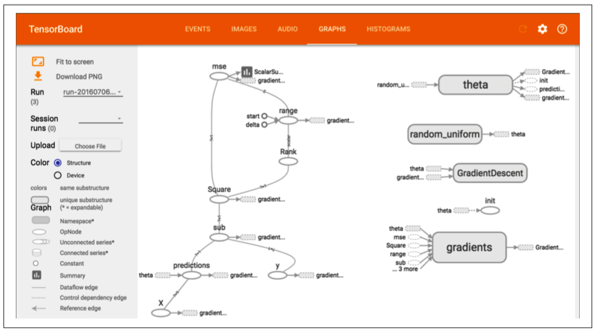
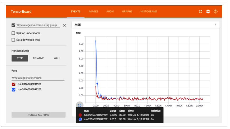
TensorBoard是一个强大的基于web的工具,它的原理是:根据保存在本地的日志数据进行绘图,可以显示图的结果和训练效果。
实现TensorBoard需要4步:
-
定义需要保存日志的文件夹
from datetime import datetime now = datetime.utcnow().strftime("%Y%m%d%H%M%S") root_logdir = "tf_logs" logdir = "{}/run-{}/".format(root_logdir, now) -
在construction phase之后,写下边的代码
mse_summary = tf.summary.scalar('MSE', mse) file_writer = tf.summary.FileWriter(logdir, tf.get_default_graph()) -
在需要写入的地方写入数据
with tf.Session() as sess: # not shown in the book sess.run(init) # not shown for epoch in range(n_epochs): # not shown for batch_index in range(n_batches): X_batch, y_batch = fetch_batch(epoch, batch_index, batch_size) if batch_index % 10 == 0: summary_str = mse_summary.eval(feed_dict={X: X_batch, y: y_batch}) step = epoch * n_batches + batch_index file_writer.add_summary(summary_str, step) sess.run(training_op, feed_dict={X: X_batch, y: y_batch}) best_theta = theta.eval() -
运行TensorBoard,键入下边命令
python3 -m tensorboard.main --logdir=tf_logs
运行后的效果图:
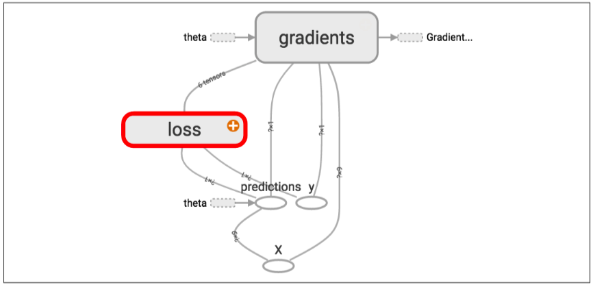
Name Scopes
当处理复杂模型的时候,比如神经网络,图中会有大量的node,就会看起来很杂乱,为了解决这个问题,可以使用TensorFlow的name scopes。
with tf.name_scope("loss") as scope:
    error = y_pred - y
    mse = tf.reduce_mean(tf.square(error), name="mse")
Modularity
Suppose you want to create a graph that adds the output of two rectified linear units(ReLU). A ReLU computes a linear function of the inputs, and outputs the result if it is positive, and 0 otherwise,
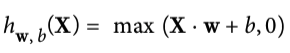
如果是两个relu,我们可以用下边的代码实现:
reset_graph()

n_features = 3
X = tf.placeholder(tf.float32, shape=(None, n_features), name="X")

w1 = tf.Variable(tf.random_normal((n_features, 1)), name="weights1")
w2 = tf.Variable(tf.random_normal((n_features, 1)), name="weights2")
b1 = tf.Variable(0.0, name="bias1")
b2 = tf.Variable(0.0, name="bias2")

z1 = tf.add(tf.matmul(X, w1), b1, name="z1")
z2 = tf.add(tf.matmul(X, w2), b2, name="z2")

relu1 = tf.maximum(z1, 0., name="relu1")
relu2 = tf.maximum(z1, 0., name="relu2")  # Oops, cut&paste error! Did you spot it?

output = tf.add(relu1, relu2, name="output")
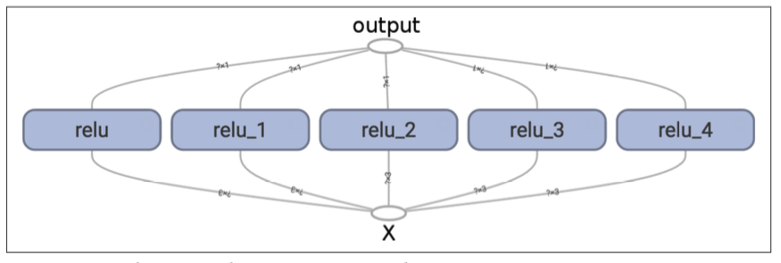
这样的代码是很糟糕的,有太多的重复代码,如果现在想扩展更多的relu,该怎么办? TensorFlow提供了add_n()方法,可以把多个值:
reset_graph()

def relu(X):
    w_shape = (int(X.get_shape()[1]), 1)
    w = tf.Variable(tf.random_normal(w_shape), name="weights")
    b = tf.Variable(0.0, name="bias")
    z = tf.add(tf.matmul(X, w), b, name="z")
    return tf.maximum(z, 0., name="relu")

n_features = 3
X = tf.placeholder(tf.float32, shape=(None, n_features), name="X")
relus = [relu(X) for i in range(5)]
output = tf.add_n(relus, name="output")
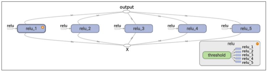
TensorFlow在创建node的时候。会为该node创建一个唯一的name,因此,我们最好在函数中使用name scopes,这样图的结构更加清晰。
def relu(X):
    with tf.name_scope("relu"):
        w_shape = (int(X.get_shape()[1]), 1)                          # not shown in the book
        w = tf.Variable(tf.random_normal(w_shape), name="weights")    # not shown
        b = tf.Variable(0.0, name="bias")                             # not shown
        z = tf.add(tf.matmul(X, w), b, name="z")                      # not shown
        return tf.maximum(z, 0., name="max")                          # not shown
Sharing Variables
还是以上边的relu为例,如果要在多个组件之中分享变量,该怎么办?有一下几个可能:
可以在relu函数中,多传递一个参数threshold,这样在调用函数的时候,就可以把该值传递到每个组件中:
reset_graph()

def relu(X, threshold):
    with tf.name_scope("relu"):
        w_shape = (int(X.get_shape()[1]), 1)                        # not shown in the book
        w = tf.Variable(tf.random_normal(w_shape), name="weights")  # not shown
        b = tf.Variable(0.0, name="bias")                           # not shown
        z = tf.add(tf.matmul(X, w), b, name="z")                    # not shown
        return tf.maximum(z, threshold, name="max")

threshold = tf.Variable(0.0, name="threshold")
X = tf.placeholder(tf.float32, shape=(None, n_features), name="X")
relus = [relu(X, threshold) for i in range(5)]
output = tf.add_n(relus, name="output")
上边的方法的缺点是,在遇到需要分享的参数有很多的时候,会不太友好,relu函数就会有很多的参数。当然,为了解决这个问题,可以给函数传递一个字典或对象也能克服这个缺点。
另一种方式是把变量保存到函数对象本身上,作为函数的属性进行传递:
reset_graph()

def relu(X):
    with tf.name_scope("relu"):
        if not hasattr(relu, "threshold"):
            relu.threshold = tf.Variable(0.0, name="threshold")
        w_shape = int(X.get_shape()[1]), 1                          # not shown in the book
        w = tf.Variable(tf.random_normal(w_shape), name="weights")  # not shown
        b = tf.Variable(0.0, name="bias")                           # not shown
        z = tf.add(tf.matmul(X, w), b, name="z")                    # not shown
        return tf.maximum(z, relu.threshold, name="max")
TensorFlow提供了get_variable()函数来获取变量,它依赖variable_scope(),变量域,
reset_graph()

with tf.variable_scope("relu"):
    threshold = tf.get_variable("threshold", shape=(),
                                initializer=tf.constant_initializer(0.0))
上边的代码,创建了一个叫做relu的变量域,因此在该域下的变量threshold的name就是relu/threshold。注意,上边的代码中,如果threshold变量如果在该代码调用之前就已经创建了,该代码会抛出异常。
如果要使用已经创建的变量,需要使用下边的代码:
with tf.variable_scope("relu", reuse=True):
    threshold = tf.get_variable("threshold")
或者:
with tf.variable_scope("relu") as scope:
    scope.reuse_variables()
    threshold = tf.get_variable("threshold")
Once reuse is set to True, it cannot be set back to False within the block. Moreover, if you define other variable scopes inside this one, they will automatically inherit reuse=True. Lastly, only variables created by get_variable() can be reused this way.
reset_graph()

def relu(X):
    with tf.variable_scope("relu", reuse=True):
        threshold = tf.get_variable("threshold")
        w_shape = int(X.get_shape()[1]), 1                          # not shown
        w = tf.Variable(tf.random_normal(w_shape), name="weights")  # not shown
        b = tf.Variable(0.0, name="bias")                           # not shown
        z = tf.add(tf.matmul(X, w), b, name="z")                    # not shown
        return tf.maximum(z, threshold, name="max")

X = tf.placeholder(tf.float32, shape=(None, n_features), name="X")
with tf.variable_scope("relu"):
    threshold = tf.get_variable("threshold", shape=(),
                                initializer=tf.constant_initializer(0.0))
relus = [relu(X) for relu_index in range(5)]
output = tf.add_n(relus, name="output")
Variables created using get_variable() are always named using the name of their variable_scope as a prefix (e.g., "relu/thres hold"), but for all other nodes (including variables created withtf.Variable()) the variable scope acts like a new name scope. In particular, if a name scope with an identical name was already cre‐ ated, then a suffix is added to make the name unique. For example, all nodes created in the preceding code (except the threshold vari‐ able) have a name prefixed with "relu_1/" to "relu_5/"
Extra material
reset_graph()

with tf.variable_scope("my_scope"):
    x0 = tf.get_variable("x", shape=(), initializer=tf.constant_initializer(0.))
    x1 = tf.Variable(0., name="x")
    x2 = tf.Variable(0., name="x")

with tf.variable_scope("my_scope", reuse=True):
    x3 = tf.get_variable("x")
    x4 = tf.Variable(0., name="x")

with tf.variable_scope("", default_name="", reuse=True):
    x5 = tf.get_variable("my_scope/x")

print("x0:", x0.op.name)
print("x1:", x1.op.name)
print("x2:", x2.op.name)
print("x3:", x3.op.name)
print("x4:", x4.op.name)
print("x5:", x5.op.name)
print(x0 is x3 and x3 is x5)

"""

x0: my_scope/x
x1: my_scope/x_1
x2: my_scope/x_2
x3: my_scope/x
x4: my_scope_1/x
x5: my_scope/x
True
"""
Exercises
-
What are the main benefits of creating a computation graph rather than directly executing the computations? What are the main drawbacks?
Main benefits and drawbacks of creating a computation graph rather than directly executing the computations:
- Main benefits:
- TensorFlow can automatically compute the gradients for you (using reverse-mode autodiff).
- TensorFlow can take care of running the operations in parallel in different threads.
- It makes it easier to run the same model across different devices.
- It simplifies introspection—for example, to view the model in TensorBoard.
- Main drawbacks:
- It makes the learning curve steeper.
- It makes step-by-step debugging harder.
- Main benefits:
-
Is the statement a_val = a.eval(session=sess) equivalent to a_val = sess.run(a)?
Yes, the statementa_val=a.eval(session=sess)is indeed equivalent toa_val = sess.run(a).
-
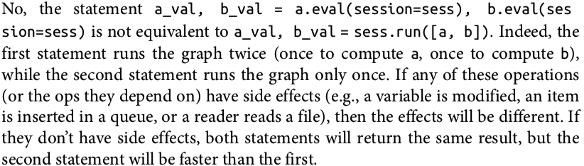
Is the statement a_val, b_val = a.eval(session=sess), b.eval(ses sion=sess) equivalent to a_val, b_val = sess.run([a, b])?
![]()
-
Can you run two graphs in the same session?
![]()
-
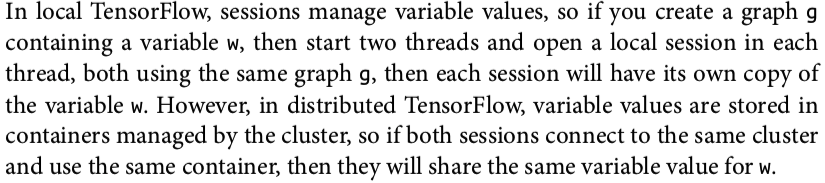
If you create a graph g containing a variable w, then start two threads and open a session in each thread, both using the same graph g, will each session have its own copy of the variable w or will it be shared?
![]()
-
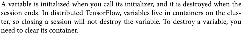
When is a variable initialized? When is it destroyed?
![]()
-
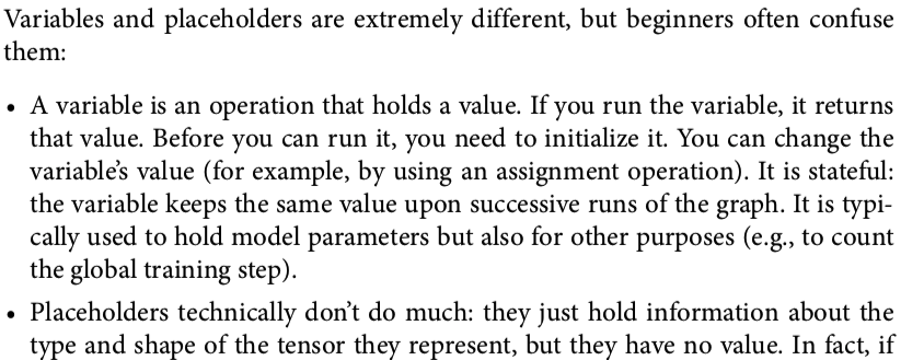
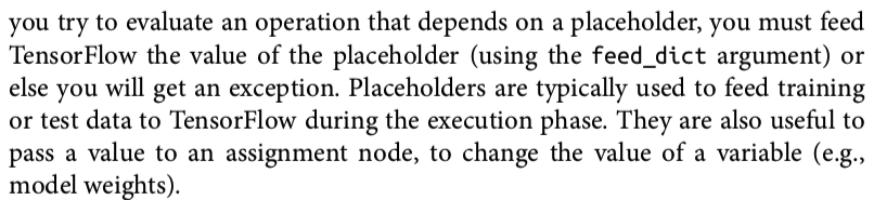
What is the difference between a placeholder and a variable?
![]()
![]()
-
What happens when you run the graph to evaluate an operation that depends on a placeholder but you don’t feed its value? What happens if the operation does not depend on the placeholder?
If you run the graph to evaluate an operation that depends on a placeholder but you don’t feed its value, you get an exception. If the operation does not depend on the placeholder, then no exception is raised.
-
When you run a graph, can you feed the output value of any operation, or just the value of placeholders?
When you run a graph, you can feed the output value of any operation, not just the value of placeholders. In practice, however, this is rather rare (it can be useful, for example, when you are caching the output of frozen layers; -
How can you set a variable to any value you want (during the execution phase)?
You can specify a variable’s initial value when constructing the graph, and it will be initialized later when you run the variable’s initializer during the execution phase. If you want to change that variable’s value to anything you want during the execution phase, then the simplest option is to create an assignment node (dur‐ ing the graph construction phase) using the tf.assign() function, passing the variable and a placeholder as parameters. During the execution phase, you can run the assignment operation and feed the variable’s new value using the place‐ holder.import tensorflow as tf x = tf.Variable(tf.random_uniform(shape=(), minval=0.0, maxval=1.0)) x_new_val = tf.placeholder(shape=(), dtype=tf.float32) x_assign = tf.assign(x, x_new_val) with tf.Session(): x.initializer.run() # random number is sampled *now* print(x.eval()) # 0.646157 (some random number) x_assign.eval(feed_dict={x_new_val: 5.0}) print(x.eval()) # 5.0 -
How many times does reverse-mode autodiff need to traverse the graph in order to compute the gradients of the cost function with regards to 10 variables? What about forward-mode autodiff? And symbolic differentiation?
Reverse-mode autodiff (implemented by TensorFlow) needs to traverse the graph only twice in order to compute the gradients of the cost function with regards to any number of variables. On the other hand, forward-mode autodiff would need to run once for each variable (so 10 times if we want the gradients with regards to 10 different variables). As for symbolic differentiation, it would build a different graph to compute the gradients, so it would not traverse the original graph at all (except when building the new gradients graph). A highly optimized symbolic differentiation system could potentially run the new gradients graph only once to compute the gradients with regards to all variables, but that new graph may be horribly complex and inefficient compared to the original graph. -
Implement Logistic Regression with Mini-batch Gradient Descent using Tensor‐ Flow. Train it and evaluate it on the moons dataset (introduced in Chapter 5). Try adding all the bells and whistles:
- Define the graph within a logistic_regression() function that can be reused easily.
- Save checkpoints using a Saver at regular intervals during training, and save the final model at the end of training.
- Restore the last checkpoint upon startup if training was interrupted.
- Define the graph using nice scopes so the graph looks good in TensorBoard.
- Add summaries to visualize the learning curves in TensorBoard.
- Try tweaking some hyperparameters such as the learning rate or the mini- batch size and look at the shape of the learning curve.

这里重点讲一下该练习题
首先我们先获取数据:
from sklearn.datasets import make_moons
m = 1000
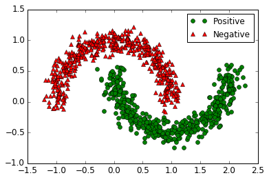
X_moons, y_moons = make_moons(m, noise=0.1, random_state=42)
看看数据的图形:
plt.plot(X_moons[y_moons == 1, 0], X_moons[y_moons == 1, 1], 'go', label="Positive")
plt.plot(X_moons[y_moons == 0, 0], X_moons[y_moons == 0, 1], 'r^', label="Negative")
plt.legend()
plt.show()
记得要为训练集X加一个偏置项:
X_moons_with_bias = np.c_[np.ones((m, 1)), X_moons]
重置y的维度
y_moons_column_vector = y_moons.reshape(-1, 1)
分隔数据为训练集和测试集
test_ratio = 0.2
test_size = int(m * test_ratio)
X_train = X_moons_with_bias[:-test_size]
X_test = X_moons_with_bias[-test_size:]
y_train = y_moons_column_vector[:-test_size]
y_test = y_moons_column_vector[-test_size:]
写一个生成batch的函数,该函数每次随机使用一定数量的数据,因此数据可能会重复
def random_batch(X_train, y_train, batch_size):
    rnd_indices = np.random.randint(0, len(X_train), batch_size)
    X_batch = X_train[rnd_indices]
    y_batch = y_train[rnd_indices]
    return X_batch, y_batch
生成模型
reset_graph()
n_inputs = 2
X = tf.placeholder(tf.float32, shape=(None, n_inputs + 1), name="X")
y = tf.placeholder(tf.float32, shape=(None, 1), name="y")
theta = tf.Variable(tf.random_uniform([n_inputs + 1, 1], -1.0, 1.0, seed=42), name="theta")
logits = tf.matmul(X, theta, name="logits")
y_proba = 1 / (1 + tf.exp(-logits))
实际上TensorFlow提供了一个 tf.sigmoid()函数
y_proba = tf.sigmoid(logits)
代价函数为:\(J(\boldsymbol{\theta}) = -\dfrac{1}{m} \sum\limits_{i=1}^{m}{\left[ y^{(i)} \log\left(\hat{p}^{(i)}\right) + (1 - y^{(i)}) \log\left(1 - \hat{p}^{(i)}\right)\right]}\)
epsilon = 1e-7  # to avoid an overflow when computing the log
loss = -tf.reduce_mean(y * tf.log(y_proba + epsilon) + (1 - y) * tf.log(1 - y_proba + epsilon))
也可以使用tf.losses.log_loss()
loss = tf.losses.log_loss(y, y_proba) # uses epsilon = 1e-7 by default
learning_rate = 0.01
optimizer = tf.train.GradientDescentOptimizer(learning_rate=learning_rate)
training_op = optimizer.minimize(loss)

init = tf.global_variables_initializer()

n_epochs = 1000
batch_size = 50
n_batches = int(np.ceil(m / batch_size))

with tf.Session() as sess:
    sess.run(init)

    for epoch in range(n_epochs):
        for batch_index in range(n_batches):
            X_batch, y_batch = random_batch(X_train, y_train, batch_size)
            sess.run(training_op, feed_dict={X: X_batch, y: y_batch})
        loss_val = loss.eval({X: X_test, y: y_test})
        if epoch % 100 == 0:
            print("Epoch:", epoch, "\tLoss:", loss_val)

    y_proba_val = y_proba.eval(feed_dict={X: X_test, y: y_test})
输出:
Epoch: 0 	Loss: 0.792602
Epoch: 100 	Loss: 0.343463
Epoch: 200 	Loss: 0.30754
Epoch: 300 	Loss: 0.292889
Epoch: 400 	Loss: 0.285336
Epoch: 500 	Loss: 0.280478
Epoch: 600 	Loss: 0.278083
Epoch: 700 	Loss: 0.276154
Epoch: 800 	Loss: 0.27552
Epoch: 900 	Loss: 0.274912
看一下模型的效果如何?
y_pred = (y_proba_val >= 0.5)
from sklearn.metrics import precision_score, recall_score

precision_score(y_test, y_pred)

"""
0.86274509803921573
"""

recall_score(y_test, y_pred)
"""
0.88888888888888884
"""
通过画图看看效果:
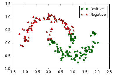
看一看出来,回归效果并不是很好,为了解决这个问题,我们首先想到,给训练数据增加新的维度,把数据映射到更高维的空间中
X_train_enhanced = np.c_[X_train,
                         np.square(X_train[:, 1]),
                         np.square(X_train[:, 2]),
                         X_train[:, 1] ** 3,
                         X_train[:, 2] ** 3]
X_test_enhanced = np.c_[X_test,
                        np.square(X_test[:, 1]),
                        np.square(X_test[:, 2]),
                        X_test[:, 1] ** 3,
                        X_test[:, 2] ** 3]
为了方便,我们定义一个函数
def logistic_regression(X, y, initializer=None, seed=42, learning_rate=0.01):
    n_inputs_including_bias = int(X.get_shape()[1])
    with tf.name_scope("logistic_regression"):
        with tf.name_scope("model"):
            if initializer is None:
                initializer = tf.random_uniform([n_inputs_including_bias, 1], -1.0, 1.0, seed=seed)
            theta = tf.Variable(initializer, name="theta")
            logits = tf.matmul(X, theta, name="logits")
            y_proba = tf.sigmoid(logits)
        with tf.name_scope("train"):
            loss = tf.losses.log_loss(y, y_proba, scope="loss")
            optimizer = tf.train.GradientDescentOptimizer(learning_rate=learning_rate)
            training_op = optimizer.minimize(loss)
            loss_summary = tf.summary.scalar('log_loss', loss)
        with tf.name_scope("init"):
            init = tf.global_variables_initializer()
        with tf.name_scope("save"):
            saver = tf.train.Saver()
    return y_proba, loss, training_op, loss_summary, init, saver
from datetime import datetime

def log_dir(prefix=""):
    now = datetime.utcnow().strftime("%Y%m%d%H%M%S")
    root_logdir = "tf_logs"
    if prefix:
        prefix += "-"
    name = prefix + "run-" + now
    return "{}/{}/".format(root_logdir, name)
真正的代码在这里
n_inputs = 2 + 4
logdir = log_dir("logreg")

X = tf.placeholder(tf.float32, shape=(None, n_inputs + 1), name="X")
y = tf.placeholder(tf.float32, shape=(None, 1), name="y")

y_proba, loss, training_op, loss_summary, init, saver = logistic_regression(X, y)

file_writer = tf.summary.FileWriter(logdir, tf.get_default_graph())
训练
n_epochs = 10001
batch_size = 50
n_batches = int(np.ceil(m / batch_size))

checkpoint_path = "/tmp/my_logreg_model.ckpt"
checkpoint_epoch_path = checkpoint_path + ".epoch"
final_model_path = "./my_logreg_model"

with tf.Session() as sess:
    if os.path.isfile(checkpoint_epoch_path):
        # if the checkpoint file exists, restore the model and load the epoch number
        with open(checkpoint_epoch_path, "rb") as f:
            start_epoch = int(f.read())
        print("Training was interrupted. Continuing at epoch", start_epoch)
        saver.restore(sess, checkpoint_path)
    else:
        start_epoch = 0
        sess.run(init)

    for epoch in range(start_epoch, n_epochs):
        for batch_index in range(n_batches):
            X_batch, y_batch = random_batch(X_train_enhanced, y_train, batch_size)
            sess.run(training_op, feed_dict={X: X_batch, y: y_batch})
        loss_val, summary_str = sess.run([loss, loss_summary], feed_dict={X: X_test_enhanced, y: y_test})
        file_writer.add_summary(summary_str, epoch)
        if epoch % 500 == 0:
            print("Epoch:", epoch, "\tLoss:", loss_val)
            saver.save(sess, checkpoint_path)
            with open(checkpoint_epoch_path, "wb") as f:
                f.write(b"%d" % (epoch + 1))

    saver.save(sess, final_model_path)
    y_proba_val = y_proba.eval(feed_dict={X: X_test_enhanced, y: y_test})
    os.remove(checkpoint_epoch_path)
看一下现在的效果
y_pred = (y_proba_val >= 0.5)
precision_score(y_test, y_pred)
"""
0.97979797979797978
"""

recall_score(y_test, y_pred)
"""
0.97979797979797978
"""
效果图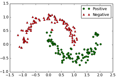
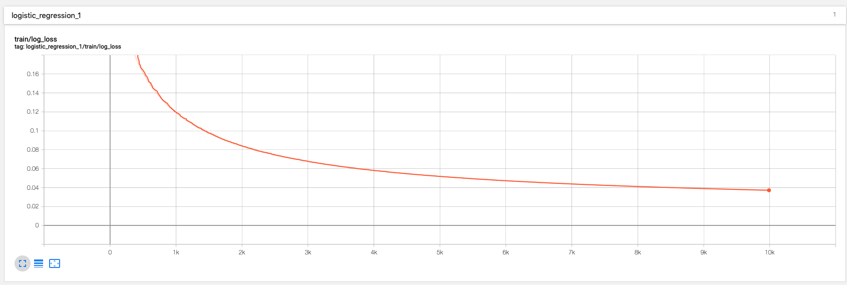
用tensorboard看一下:
上边代码中的参数,还可以优化,可以使用grid search和randomized search,我们下边演示使用randomized search方法,我们需要优化的参数是batch_size和learning_rate
from scipy.stats import reciprocal

n_search_iterations = 10

for search_iteration in range(n_search_iterations):
    batch_size = np.random.randint(1, 100)
    learning_rate = reciprocal(0.0001, 0.1).rvs(random_state=search_iteration)

    n_inputs = 2 + 4
    logdir = log_dir("logreg")

    print("Iteration", search_iteration)
    print("  logdir:", logdir)
    print("  batch size:", batch_size)
    print("  learning_rate:", learning_rate)
    print("  training: ", end="")

    reset_graph()

    X = tf.placeholder(tf.float32, shape=(None, n_inputs + 1), name="X")
    y = tf.placeholder(tf.float32, shape=(None, 1), name="y")

    y_proba, loss, training_op, loss_summary, init, saver = logistic_regression(
        X, y, learning_rate=learning_rate)

    file_writer = tf.summary.FileWriter(logdir, tf.get_default_graph())

    n_epochs = 10001
    n_batches = int(np.ceil(m / batch_size))

    final_model_path = "./my_logreg_model_%d" % search_iteration

    with tf.Session() as sess:
        sess.run(init)

        for epoch in range(n_epochs):
            for batch_index in range(n_batches):
                X_batch, y_batch = random_batch(X_train_enhanced, y_train, batch_size)
                sess.run(training_op, feed_dict={X: X_batch, y: y_batch})
            loss_val, summary_str = sess.run([loss, loss_summary], feed_dict={X: X_test_enhanced, y: y_test})
            file_writer.add_summary(summary_str, epoch)
            if epoch % 500 == 0:
                print(".", end="")

        saver.save(sess, final_model_path)

        print()
        y_proba_val = y_proba.eval(feed_dict={X: X_test_enhanced, y: y_test})
        y_pred = (y_proba_val >= 0.5)

        print("  precision:", precision_score(y_test, y_pred))
        print("  recall:", recall_score(y_test, y_pred))
输出如下
Iteration 0
  logdir: tf_logs/logreg-run-20170606195328/
  batch size: 19
  learning_rate: 0.00443037524522
  training: .....................
  precision: 0.979797979798
  recall: 0.979797979798
Iteration 1
  logdir: tf_logs/logreg-run-20170606195605/
  batch size: 80
  learning_rate: 0.00178264971514
  training: .....................
  precision: 0.969696969697
  recall: 0.969696969697
Iteration 2
  logdir: tf_logs/logreg-run-20170606195646/
  batch size: 73
  learning_rate: 0.00203228544324
  training: .....................
  precision: 0.969696969697
  recall: 0.969696969697
Iteration 3
  logdir: tf_logs/logreg-run-20170606195730/
  batch size: 6
  learning_rate: 0.00449152382514
  training: .....................
  precision: 0.980198019802
  recall: 1.0
Iteration 4
  logdir: tf_logs/logreg-run-20170606200523/
  batch size: 24
  learning_rate: 0.0796323472178
  training: .....................
  precision: 0.980198019802
  recall: 1.0
Iteration 5
  logdir: tf_logs/logreg-run-20170606200726/
  batch size: 75
  learning_rate: 0.000463425058329
  training: .....................
  precision: 0.912621359223
  recall: 0.949494949495
Iteration 6
  logdir: tf_logs/logreg-run-20170606200810/
  batch size: 86
  learning_rate: 0.0477068184194
  training: .....................
  precision: 0.98
  recall: 0.989898989899
Iteration 7
  logdir: tf_logs/logreg-run-20170606200851/
  batch size: 87
  learning_rate: 0.000169404470952
  training: .....................
  precision: 0.888888888889
  recall: 0.808080808081
Iteration 8
  logdir: tf_logs/logreg-run-20170606200932/
  batch size: 61
  learning_rate: 0.0417146119941
  training: .....................
  precision: 0.980198019802
  recall: 1.0
Iteration 9
  logdir: tf_logs/logreg-run-20170606201026/
  batch size: 92
  learning_rate: 0.000107429229684
  training: .....................
  precision: 0.882352941176
  recall: 0.757575757576
很直观的就发现了当前的最优参数,看看tensorboard
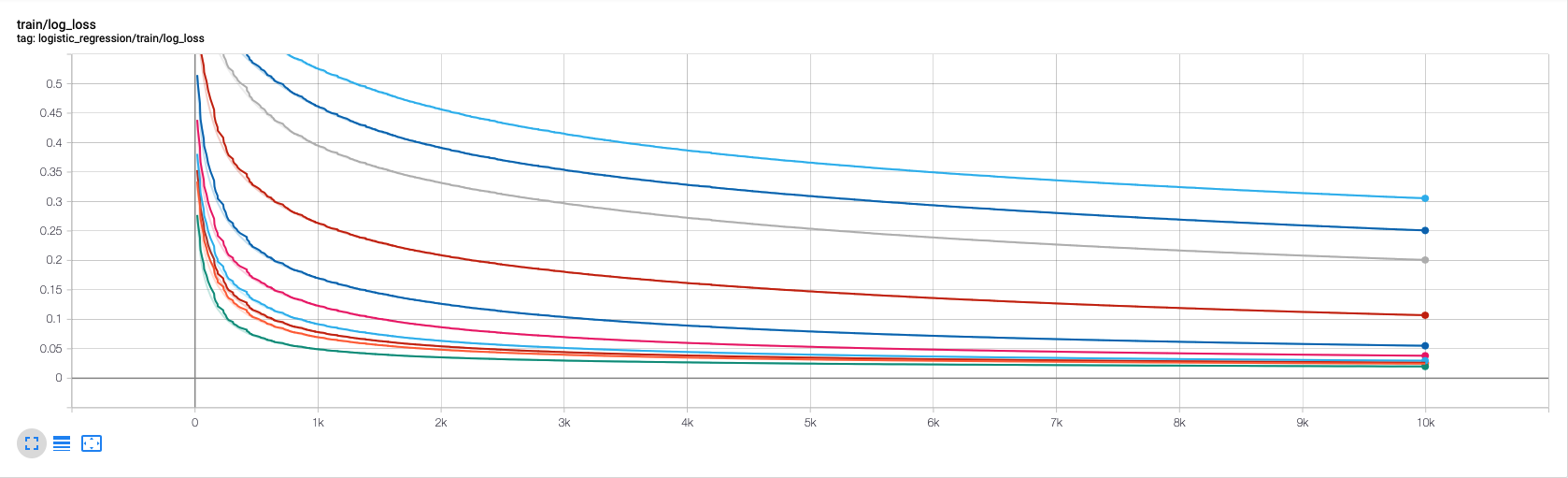
可以看出,不同参数,学习曲线是不同的。

 浙公网安备 33010602011771号