
注:本文为 “Dirac‘s Delta Function” 相关合辑。
英文引文,机翻未校。
如有内容异常,请看原文。
What Exactly is Dirac’s Delta Function?
狄拉克 δ δδ函数究竟是什么?
2025-08-29 00:00:00
1. Introduction: “Convenient Notation”
引言:“便捷符号”
Approaching a Dirac delta function
趋近于狄拉克δ δδ 函数
In Dirac’sPrinciples of Quantum Mechanicspublished in 1930 he introduced a “convenient notation” he referred to as a “delta function” which he treated as a continuum analog to the discrete Kronecker delta.
在狄拉克于 1930 年出版的《量子力学原理》(Principles of Quantum Mechanics)一书中,他引入了一种“便捷符号”,并将其称为“δ δδ函数”,还把这种δ δδ函数视为离散克罗内克δ符号在连续情形下的类似物。
The Kronecker delta is simply the indexed components of the identity operator in matrix algebra:
在矩阵代数中,克罗内克δ符号本质上就是单位算子的带指标分量,其定义如下:
δ i j = { 1 if i = j 0 if i ≠ j \delta_{ij} = \begin{cases} 1 & \text{if } i = j \\ 0 & \text{if } i \neq j \end{cases}δij={10if i=jif i=j
The key utility of the Kronecker delta is its occurrence in summations:
克罗内克δ符号的核心用途体现在求和运算中,例如:
∑ i A i δ i j = A j \sum_{i} A_i \delta_{ij} = A_j∑iAiδij=Aj(对指标 i ii求和后,结果为A j A_jAj)
Similarly Dirac’s delta function is principally defined as it occurs in integrals:
与之类似,狄拉克δ δδ函数的定义也主要依托其在积分中的表现,其核心积分定义为:
∫ − ∞ ∞ f ( x ) δ ( x ) d x = f ( 0 ) \int_{-\infty}^{\infty} f(x) \delta(x) dx = f(0)∫−∞∞f(x)δ(x)dx=f(0)(其中 f ( x ) f(x)f(x) 是在 x = 0 x = 0x=0处连续的函数)
Viewed another way the delta function allows you to evaluate the function at zero (and, via translations, elsewhere) by integrating:
换一种角度理解,利用积分运算,δ δδ函数能让大家求出函数在x = 0 x = 0x=0处的取值(通过平移,还能求出函数在其他点的取值),平移后的积分形式为:
∫ − ∞ ∞ f ( x ) δ ( x − a ) d x = f ( a ) \int_{-\infty}^{\infty} f(x) \delta(x - a) dx = f(a)∫−∞∞f(x)δ(x−a)dx=f(a)(其中 a aa为任意实数,f ( x ) f(x)f(x) 在 x = a x = ax=a 处连续)
The problem is that no such function exists, as such, in the space of real functions.
但难题在于,在实函数空间中,并不存在这样一种满足上述积分性质的函数。
The delta “function” is not, in fact, a function which is why Dirac referred to it as “convenient notation”.
事实上,此种δ“函数”根本不是传统意义上的函数,这也正是狄拉克将其称为“便捷符号”的原因。
This begs the question, “So what does this convenient notation represent?” For the mathematician this means “Where’s the rigor?” and for the physicist it means “Will using this give me well defined predictions?” This article points to some of the mathematical contexts in which Dirac’s convenient notation has been given proper mathematical meaning.
这就引出了一个挑战:“此种便捷符号究竟代表什么?”对数学家而言,该问题等价于“其严格的数学基础在哪里?”;对物理学家而言,则是“使用这个符号能否得出明确的预测结果?”。本文将介绍一些数学框架,在这些框架中,狄拉克提出的这一便捷符号被赋予了严谨的数学意义。
2. Riemann-Stieltjes Integrals
黎曼-斯蒂尔杰斯积分
We can formally define the Riemann-Stieltjes (R-S) Integral:
大家可能正式定义黎曼-斯蒂尔杰斯(R-S)积分。对于性质良好的实值函数f ( x ) f(x)f(x) 和 g ( x ) g(x)g(x),其 R-S 积分定义为:
∫ a b f ( x ) d g ( x ) \int_{a}^{b} f(x) dg(x)∫abf(x)dg(x)
for well behaved real functionsf ff and g ggin the same way we defined our Riemann integrals, as limits of (modified) Riemann sums.
其定义方式与黎曼积分类似,都是通过(修正后的)黎曼和的极限来定义,即:
∫ a b f ( x ) d g ( x ) = lim n → ∞ ∑ k = 1 n f ( x k ∗ ) [ g ( x k ) − g ( x k − 1 ) ] \int_{a}^{b} f(x) dg(x) = \lim_{n \to \infty} \sum_{k=1}^{n} f(x_k^*) [g(x_k) - g(x_{k-1})]∫abf(x)dg(x)=limn→∞∑k=1nf(xk∗)[g(xk)−g(xk−1)](其中 x 0 = a , x n = b x_0 = a, x_n = bx0=a,xn=b,x k ∗ x_k^*xk∗ 是区间 [ x k − 1 , x k ] [x_{k-1}, x_k][xk−1,xk]内的任意一点,当分割区间的最大长度趋近于 0 时取极限)
Where g ggis differentiable we can also prove integration by parts holds and express those R-S integrals as simple Riemann Integrals:
当 g ( x ) g(x)g(x)通过可微时,我们能够证明分部积分公式对 R-S 积分成立,并且能将 R-S 积分转化为简单的黎曼积分:
∫ a b f ( x ) d g ( x ) = f ( b ) g ( b ) − f ( a ) g ( a ) − ∫ a b g ( x ) d f ( x ) \int_{a}^{b} f(x) dg(x) = f(b)g(b) - f(a)g(a) - \int_{a}^{b} g(x) df(x)∫abf(x)dg(x)=f(b)g(b)−f(a)g(a)−∫abg(x)df(x)(分部积分公式)
∫ a b f ( x ) d g ( x ) = ∫ a b f ( x ) g ′ ( x ) d x \int_{a}^{b} f(x) dg(x) = \int_{a}^{b} f(x) g'(x) dx∫abf(x)dg(x)=∫abf(x)g′(x)dx(当 g ′ ( x ) g'(x)g′(x)连续时,R-S 积分可转化为黎曼积分)
This is valid even when the derivative ofg ggis problematic in the interval of integration.
即便 g ( x ) g(x)g(x)的导数在积分区间内存在“问题”(如不连续、不存在),上述 R-S 积分的定义仍然有效。
Of course identities are two way streets and we rewrite apparent Riemann integrals as well defined R-S integrals.
当然,恒等式具有双向性,我们也可以将看似是黎曼积分的表达式改写为定义严谨的 R-S 积分。例如,若令g ( x ) = x g(x) = xg(x)=x,则 ∫ a b f ( x ) d x = ∫ a b f ( x ) d g ( x ) \int_{a}^{b} f(x) dx = \int_{a}^{b} f(x) dg(x)∫abf(x)dx=∫abf(x)dg(x),此时黎曼积分就成为了 R-S 积分的一种特殊情况。
This is an improvement because Riemann-Stieltjes integrals have a broader domain of application.
这是一种改进,因为黎曼-斯蒂尔杰斯积分的适用范围更广泛,它能处理被积函数或“积分变量函数”(即g ( x ) g(x)g(x))存在间断的情况,而传统黎曼积分对此无能为力。
3. The Dirac delta function as the “derivative” of the Heaviside step function
作为亥维赛阶跃函数“导数”的狄拉克δ δδ 函数
Consider the functionH ( x ) H(x)H(x)such that:
考虑函数 H ( x ) H(x)H(x)(即亥维赛阶跃函数),其定义为:
H ( x ) = { 0 if x < 0 1 if x > 0 H(x) = \begin{cases} 0 & \text{if } x < 0 \\ 1 & \text{if } x > 0 \end{cases}H(x)={01if x<0if x>0(注:H ( 0 ) H(0)H(0)的取值通常定义为 0、1 或 1/2,不影响积分结果)
This is the Heaviside step function which is also denotedθ ( x ) \theta(x)θ(x)in many texts.
这就是亥维赛阶跃函数,在许多文献中也用符号θ ( x ) \theta(x)θ(x) 表示。
Now consider the R-S integral:
现在考虑如下 R-S 积分:
∫ − ∞ ∞ f ( x ) d H ( x ) \int_{-\infty}^{\infty} f(x) dH(x)∫−∞∞f(x)dH(x)
Careful evaluation of the limit of the modified Riemann sum will yield zero if0 00is outside the open interval( a , b ) (a, b)(a,b)(where the integral is taken over[ a , b ] [a, b][a,b]). But for0 ∈ ( a , b ) 0 \in (a, b)0∈(a,b)we getf ( 0 ) f(0)f(0).
若 0 不在积分区间[ a , b ] [a, b][a,b]对应的开区间( a , b ) (a, b)(a,b)内,通过仔细计算修正黎曼和的极限,该积分结果为 0;若0 ∈ ( a , b ) 0 \in (a, b)0∈(a,b),则积分结果为f ( 0 ) f(0)f(0)。
We can of course translate the step function to evaluatef ffat any real valuea aa:
当然,大家可以对阶跃函数进行平移,从而求出函数f ( x ) f(x)f(x) 在任意实数 a aa处的取值,平移后的积分形式为:
∫ − ∞ ∞ f ( x ) d H ( x − a ) = f ( a ) \int_{-\infty}^{\infty} f(x) dH(x - a) = f(a)∫−∞∞f(x)dH(x−a)=f(a)(其中 H ( x − a ) H(x - a)H(x−a)是平移后的亥维赛阶跃函数,满足H ( x − a ) = 0 H(x - a) = 0H(x−a)=0(x < a x < ax<a)、H ( x − a ) = 1 H(x - a) = 1H(x−a)=1(x > a x > ax>a))
We thus get the exact same behavior as Dirac’s “convenient notation” and we can use this as the definition of that notation:
由此可见,该 R-S 积分的性质与狄拉克“便捷符号”(即δ δδ函数)的性质完全一致,因此我们可以将其作为δ δδ函数符号的定义:
∫ − ∞ ∞ f ( x ) δ ( x − a ) d x = ∫ − ∞ ∞ f ( x ) d H ( x − a ) \int_{-\infty}^{\infty} f(x) \delta(x - a) dx = \int_{-\infty}^{\infty} f(x) dH(x - a)∫−∞∞f(x)δ(x−a)dx=∫−∞∞f(x)dH(x−a)
Hence we often speak of the Dirac delta function as the “derivative” of the Heaviside step function.
因此,我们常说狄拉克δ δδ函数是亥维赛阶跃函数的“导数”——这里的“导数”并非传统意义上的可微性,而是基于 R-S 积分的“广义导数”。
The use of R-S integrals does not however deal directly with other equally convenient notations. We can for example consider “derivatives” of Dirac’s delta function which have the defining property of evaluating the n-th derivative (with sign changes) of a function:
然而,黎曼-斯蒂尔杰斯积分无法直接处理δ δδ通过函数的“导数”等其他便捷符号。例如,我们能够定义δ δδ函数的“n 阶导数”δ ( n ) ( x − a ) \delta^{(n)}(x - a)δ(n)(x−a),其核心性质是能通过积分求出函数f ( x ) f(x)f(x) 在 a aa处的 n 阶导数(并伴随符号变化),即:
∫ − ∞ ∞ f ( x ) δ ( n ) ( x − a ) d x = ( − 1 ) n f ( n ) ( a ) \int_{-\infty}^{\infty} f(x) \delta^{(n)}(x - a) dx = (-1)^n f^{(n)}(a)∫−∞∞f(x)δ(n)(x−a)dx=(−1)nf(n)(a)(其中 f ( n ) ( a ) f^{(n)}(a)f(n)(a) 表示 f ( x ) f(x)f(x) 在 x = a x = ax=a处的 n 阶导数,且f ( x ) f(x)f(x)具有足够阶数的连续性)
One can obtain this result by repeatedly applying integration by parts to peel off the formal derivatives ofδ \deltaδuntil one has a valid Riemann-Stieltjes integral.
通过对上述积分反复应用分部积分法,逐步“剥离”δ δδ函数的形式导数,最终可将其转化为实用的黎曼-斯蒂尔杰斯积分,从而得到上述结果。例如,对于一阶导数δ ′ ( x − a ) \delta'(x - a)δ′(x−a),分部积分后可得:
∫ − ∞ ∞ f ( x ) δ ′ ( x − a ) d x = − ∫ − ∞ ∞ f ′ ( x ) δ ( x − a ) d x = − f ′ ( a ) \int_{-\infty}^{\infty} f(x) \delta'(x - a) dx = - \int_{-\infty}^{\infty} f'(x) \delta(x - a) dx = -f'(a)∫−∞∞f(x)δ′(x−a)dx=−∫−∞∞f′(x)δ(x−a)dx=−f′(a)
This suggests we can extend the definition, say Extended Riemann-Stieltjes Integrals. However, this approach has now been supplanted with the more general Lebesgue integration.
这提示我们可以扩展 R-S 积分的定义(即“推广的黎曼-斯蒂尔杰斯积分”),但如今此种方法已被更具一般性的勒贝格积分所取代。
Dirac’s delta function is considered (notation for) a distribution. Specifically it is (and its derivatives are) expressed in terms of the Radon-Nikodym derivative(s) of the measure defined by the Heaviside step function.
在现代数学中,狄拉克δ δδ函数被视为一种“广义函数”(或“分布”)的符号。具体而言,δ δδ函数及其导数可通过亥维赛阶跃函数所定义的测度的拉东-尼科迪姆导数来表示,这为其提供了严格的测度论基础。
There is a more operational approach to understanding Dirac’s delta function in terms of how it is actually being used.
除了上述数学框架,我们还可以从“实际应用”的角度出发,通过δ δδ函数的使用方式来直观理解它,这是一种更偏向“操作性”的理解方法。
4. Vectors, dual vectors, and Riesz’s representation theorem
向量、对偶向量与里斯表示定理
Recall that for finite dimensional vector spaces, sayR n \mathbb{R}^nRn, the set of linear functionals (linear mappings from vectors to scalars) forms its own vector space, the dual space( R n ) ∗ (\mathbb{R}^n)^*(Rn)∗of equal dimension.
回顾线性代数知识:对于有限维向量空间(如R n \mathbb{R}^nRn,即 n 维实向量空间),所有线性泛函(将向量映射到标量的线性映射)构成的集合本身也是一个向量空间,称为“对偶空间”,记为( R n ) ∗ (\mathbb{R}^n)^*(Rn)∗,且对偶空间的维数与原空间相同(均为 n)。
For infinite dimensional spaces this is also the case except the dimension of the dual space may be a higher order of infinity.
对于无限维向量空间,线性泛函的集合同样构成对偶空间,但对偶空间的维数可能是“更高阶的无穷大”(即对偶空间与原空间不“同构”)。
This comes into play when the vector space also possesses an inner product (for example the dot product) in such case the Riesz Representation applies.
当向量空间还配备了内积(例如欧氏空间中的点积)时,上述对偶空间的性质会进一步简化,此时“里斯表示定理”便可以发挥作用。
Riesz Representation Theorem: For any Hilbert spaceH \mathcal{H}Hwith inner product⟨ ⋅ , ⋅ ⟩ \langle \cdot, \cdot \rangle⟨⋅,⋅⟩, for every bounded linear functionalL : H → C L: \mathcal{H} \to \mathbb{C}L:H→C (or R \mathbb{R}Rfor real Hilbert spaces) there exists a unique vectorv L ∈ H v_L \in \mathcal{H}vL∈Hsuch that:
里斯表示定理:对于任意配备内积⟨ ⋅ , ⋅ ⟩ \langle \cdot, \cdot \rangle⟨⋅,⋅⟩的希尔伯特空间H \mathcal{H}H(希尔伯特空间是完备的内积空间),对每一个有界线性泛函L : H → C L: \mathcal{H} \to \mathbb{C}L:H→C(若为实希尔伯特空间,则映射到R \mathbb{R}R),都存在唯一的向量v L ∈ H v_L \in \mathcal{H}vL∈H,使得:
L ( u ) = ⟨ u , v L ⟩ L(u) = \langle u, v_L \rangleL(u)=⟨u,vL⟩for allu ∈ H u \in \mathcal{H}u∈H
对所有 u ∈ H u \in \mathcal{H}u∈H,都有 L ( u ) = ⟨ u , v L ⟩ L(u) = \langle u, v_L \rangleL(u)=⟨u,vL⟩
(We here use the convention that complex inner products are linear on the 2nd argument whereas many texts reverse this. In general it is linear in one and conjugate linear in the other since⟨ u , α v + β w ⟩ = α ⟨ u , v ⟩ + β ⟨ u , w ⟩ \langle u, \alpha v + \beta w \rangle = \alpha \langle u, v \rangle + \beta \langle u, w \rangle⟨u,αv+βw⟩=α⟨u,v⟩+β⟨u,w⟩ and ⟨ α u + β v , w ⟩ = α ‾ ⟨ u , w ⟩ + β ‾ ⟨ v , w ⟩ \langle \alpha u + \beta v, w \rangle = \overline{\alpha} \langle u, w \rangle + \overline{\beta} \langle v, w \rangle⟨αu+βv,w⟩=α⟨u,w⟩+β⟨v,w⟩.)
(本文采用的约定是:复内积对第二个变元是线性的,而许多文献会采用相反的约定(对第一个变元线性)。一般而言,内积对一个变元是线性的,对另一个变元是“共轭线性”的,即满足⟨ u , α v + β w ⟩ = α ⟨ u , v ⟩ + β ⟨ u , w ⟩ \langle u, \alpha v + \beta w \rangle = \alpha \langle u, v \rangle + \beta \langle u, w \rangle⟨u,αv+βw⟩=α⟨u,v⟩+β⟨u,w⟩(对第二个变元线性)和⟨ α u + β v , w ⟩ = α ‾ ⟨ u , w ⟩ + β ‾ ⟨ v , w ⟩ \langle \alpha u + \beta v, w \rangle = \overline{\alpha} \langle u, w \rangle + \overline{\beta} \langle v, w \rangle⟨αu+βv,w⟩=α⟨u,w⟩+β⟨v,w⟩(对第一个变元共轭线性),其中α ‾ \overline{\alpha}α 表示 α \alphaα的复共轭。)
Now if we are working in real vector spaces the inner product is essentially a “dot product” so we can say that we identify the bounded linear functionalL LLwith the operation, of dotting the argument vectoru uu with v L v_LvL.
若大家考虑的是实向量空间,此时内积本质上就是“点积”(如R n \mathbb{R}^nRn 中的 ⟨ u , v ⟩ = u ⋅ v = u 1 v 1 + u 2 v 2 + ⋯ + u n v n \langle u, v \rangle = u \cdot v = u_1 v_1 + u_2 v_2 + \dots + u_n v_n⟨u,v⟩=u⋅v=u1v1+u2v2+⋯+unvn),因此我们能够将有界线性泛函L LL 与“将向量 u uu 和 v L v_LvL做点积”这一运算等同起来——即每个有界线性泛函都对应一个“代表向量”v L v_LvL,泛函的作用可通过点积实现。
A bounded linear functional (on an inner product space) is a functional such that its absolute value is bounded over the set of vectors with unit norm.
内积空间上的“有界线性泛函”是指:对于所有范数为 1 的向量u uu(即 ∥ u ∥ = 1 \|u\| = 1∥u∥=1),泛函值的绝对值都有上界,即存在常数M > 0 M > 0M>0,使得 ∣ L ( u ) ∣ ≤ M |L(u)| \leq M∣L(u)∣≤M 对所有 ∥ u ∥ = 1 \|u\| = 1∥u∥=1 成立。
For spaces of finite dimension, this is always the case. This boundedness condition is something we only have to worry about in infinite-dimensional spaces.
在有限维向量空间中,所有线性泛函都是有界的——这是有限维空间的固有性质,无需额外验证。而在无限维空间中,线性泛函可能是无界的,因此“有界性”成为了需要特别关注的条件。
Because of this theorem, when teaching introductory vectors and linear algebra, there is no pragmatic need to bring up dual spaces. It is mostly sufficient to express any dual vector operation in terms of a vector and dot product.
正是由于里斯表示定理的存在,在教授基础向量和线性代数(通常以有限维空间为主)时,实际上无需引入对偶空间的概念——缘于所有对偶向量(即线性泛函)的作用都可能借助“代表向量”和点积来表示,此种方式更直观、更易理解。
The problems occur when we need to go beyond finite dimensional spaces. We then need to deal with those unbounded linear functionals explicitly when they are used.
当研究范围超出有限维空间(如进入无限维函数空间)时,问题就出现了:此时会遇到无界线性泛函,而里斯表示定理对无界泛函失效,因此我们必须明确地处理这些无界线性泛函。
5. The “dot product” of two functions
两个函数的“点积”
Now consider the vector space of all real valued functions. To implement an inner product and norm we have to restrict to a subspace where those operations are finite but we can gloss over such details for this discussion.
现在考虑“所有实值函数构成的向量空间”——但这个空间过于宽泛,若要定义内积和范数,我们需要将其限制在一个“子空间”内,确保内积和范数的计算结果是有限的(即不发散)。为简化讨论,我们先暂时忽略这些限制条件,聚焦于内积的定义形式。
We define the following inner (dot) product between two suitable vectors (functions)f ff and g gg:
对于两个“合适的”向量(即函数)f ( x ) f(x)f(x) 和 g ( x ) g(x)g(x),我们定义如下内积(也可称为“函数的点积”):
⟨ f , g ⟩ = ∫ − ∞ ∞ f ( x ) g ( x ) d x \langle f, g \rangle = \int_{-\infty}^{\infty} f(x) g(x) dx⟨f,g⟩=∫−∞∞f(x)g(x)dx
Note that with an inner product we also have a norm and can thus normalize our functions (construct “unit vectors”).
通过,有了内积后,我们能够经过内积定义范数:就是需要注意的∥ f ∥ = ⟨ f , f ⟩ \|f\| = \sqrt{\langle f, f \rangle}∥f∥=⟨f,f⟩通过。利用范数,我们能够对函数进行“归一化”(即使其范数为 1),得到“单位向量”(即单位函数)。
So for example forf ( x ) = e − x 2 / 2 f(x) = e^{-x^2/2}f(x)=e−x2/2 and g ( x ) = e − x 2 / 2 g(x) = e^{-x^2/2}g(x)=e−x2/2we have:
例如,取函数f ( x ) = e − x 2 / 2 f(x) = e^{-x^2/2}f(x)=e−x2/2 和 g ( x ) = e − x 2 / 2 g(x) = e^{-x^2/2}g(x)=e−x2/2,则内积为:
⟨ f , g ⟩ = ∫ − ∞ ∞ e − x 2 / 2 ⋅ e − x 2 / 2 d x = ∫ − ∞ ∞ e − x 2 d x = π \langle f, g \rangle = \int_{-\infty}^{\infty} e^{-x^2/2} \cdot e^{-x^2/2} dx = \int_{-\infty}^{\infty} e^{-x^2} dx = \sqrt{\pi}⟨f,g⟩=∫−∞∞e−x2/2⋅e−x2/2dx=∫−∞∞e−x2dx=π(这是高斯积分的经典结果)
and
因此,f ( x ) f(x)f(x) 的范数为:
∥ f ∥ = ⟨ f , f ⟩ = π = π 1 / 4 \|f\| = \sqrt{\langle f, f \rangle} = \sqrt{\sqrt{\pi}} = \pi^{1/4}∥f∥=⟨f,f⟩=π=π1/4
Hence,f ~ ( x ) = f ( x ) ∥ f ∥ = e − x 2 / 2 π 1 / 4 \tilde{f}(x) = \frac{f(x)}{\|f\|} = \frac{e^{-x^2/2}}{\pi^{1/4}}f~(x)=∥f∥f(x)=π1/4e−x2/2is a normalized function i.e. a “unit vector” in this space.
因此,函数 f ~ ( x ) = f ( x ) ∥ f ∥ = e − x 2 / 2 π 1 / 4 \tilde{f}(x) = \frac{f(x)}{\|f\|} = \frac{e^{-x^2/2}}{\pi^{1/4}}f~(x)=∥f∥f(x)=π1/4e−x2/2是归一化的,即该函数空间中的“单位向量”(满足∥ f ~ ∥ = 1 \|\tilde{f}\| = 1∥f~∥=1)。
For many functions the integral defining their norm will diverge or just can’t be defined. So, we toss those cases out and restrict our considerations to the set of functions of finite norm.
对于许多函数而言,通过上述积分定义的范数会发散(如f ( x ) = 1 f(x) = 1f(x)=1,其范数 ∥ f ∥ = ∫ − ∞ ∞ 1 d x \|f\| = \int_{-\infty}^{\infty} 1 dx∥f∥=∫−∞∞1dx发散),或根本无法定义。因此,大家需要排除这些函数,将研究范围限制在“范数有限的函数”构成的集合上。
This again defines a vector space, the space of square integrable functions. Since the norm is defined in terms of an inner product this is an inner product space.
该“范数有限的函数集合”本身也是一个向量空间,称为“平方可积函数空间”,记为L 2 ( R ) L^2(\mathbb{R})L2(R)通过内积定义的,因此就是(表示在实轴上平方可积的函数)。由于其范数L 2 ( R ) L^2(\mathbb{R})L2(R)也是一个内积空间(且是完备的,属于希尔伯特空间)。
6. The evaluation functional
赋值泛函
Unfortunately, for unbounded linear functionals the Riesz’s representation theorem fails. One might think this is not too important. But, one will be surprised to see how often an important operation involves a linear functional which is unbounded.
遗憾的是,里斯表示定理仅适用于有界线性泛函,对无界线性泛函失效。有人可能认为无界泛函并不重要,但实际情况是:在许多关键运算中,都会涉及无界线性泛函,这一点可能出人意料。
We can define the set of evaluation functionals,L a : L 2 ( R ) → R L_a: L^2(\mathbb{R}) \to \mathbb{R}La:L2(R)→R, such thatL a ( f ) = f ( a ) L_a(f) = f(a)La(f)=f(a).
我们可以定义一类重要的无界线性泛函——“赋值泛函”,记为L a : L 2 ( R ) → R L_a: L^2(\mathbb{R}) \to \mathbb{R}La:L2(R)→R,其作用是“求函数f ( x ) f(x)f(x) 在 x = a x = ax=a处的取值”,即L a ( f ) = f ( a ) L_a(f) = f(a)La(f)=f(a)(其中 a aa是任意实数,f ∈ L 2 ( R ) f \in L^2(\mathbb{R})f∈L2(R))。
They are functionals in that they map functions to numbers.
赋值泛函之所以是“泛函”,是因为它将函数(向量)映射到了标量(实数)。
That they are linear is trivial:
赋值泛函的“线性”性质很容易验证:
L a ( α f + β g ) = ( α f + β g ) ( a ) = α f ( a ) + β g ( a ) = α L a ( f ) + β L a ( g ) L_a(\alpha f + \beta g) = (\alpha f + \beta g)(a) = \alpha f(a) + \beta g(a) = \alpha L_a(f) + \beta L_a(g)La(αf+βg)=(αf+βg)(a)=αf(a)+βg(a)=αLa(f)+βLa(g)(其中 α , β \alpha, \betaα,β是任意实数,f , g ∈ L 2 ( R ) f, g \in L^2(\mathbb{R})f,g∈L2(R))
That they are unbounded (inL 2 ( R ) L^2(\mathbb{R})L2(R)) is fairly easy to demonstrate. For example, the square root of the probability density function for a normal random variable with meana aaand standard deviationσ \sigmaσ is f σ ( x ) = ( 1 σ 2 π ) 1 / 2 e − ( x − a ) 2 / ( 4 σ 2 ) f_{\sigma}(x) = \left( \frac{1}{\sigma \sqrt{2\pi}} \right)^{1/2} e^{-(x - a)^2/(4\sigma^2)}fσ(x)=(σ2π1)1/2e−(x−a)2/(4σ2); it has unit norm,∥ f σ ∥ 2 = ∫ − ∞ ∞ f σ ( x ) 2 d x = ∫ − ∞ ∞ 1 σ 2 π e − ( x − a ) 2 / ( 2 σ 2 ) d x = 1 \|f_{\sigma}\|^2 = \int_{-\infty}^{\infty} f_{\sigma}(x)^2 dx = \int_{-\infty}^{\infty} \frac{1}{\sigma \sqrt{2\pi}} e^{-(x - a)^2/(2\sigma^2)} dx = 1∥fσ∥2=∫−∞∞fσ(x)2dx=∫−∞∞σ2π1e−(x−a)2/(2σ2)dx=1(the total probability).
赋值泛函在 L 2 ( R ) L^2(\mathbb{R})L2(R)“无界的”,这一点也很容易证明。例如,考虑均值为就是中a aa、标准差为 σ \sigmaσ的正态分布概率密度函数,其平方根为f σ ( x ) = ( 1 σ 2 π ) 1 / 2 e − ( x − a ) 2 / ( 4 σ 2 ) f_{\sigma}(x) = \left( \frac{1}{\sigma \sqrt{2\pi}} \right)^{1/2} e^{-(x - a)^2/(4\sigma^2)}fσ(x)=(σ2π1)1/2e−(x−a)2/(4σ2)。该函数的范数为 1(因为概率密度函数的积分等于 1,即∥ f σ ∥ 2 = ∫ − ∞ ∞ f σ ( x ) 2 d x = ∫ − ∞ ∞ 1 σ 2 π e − ( x − a ) 2 / ( 2 σ 2 ) d x = 1 \|f_{\sigma}\|^2 = \int_{-\infty}^{\infty} f_{\sigma}(x)^2 dx = \int_{-\infty}^{\infty} \frac{1}{\sigma \sqrt{2\pi}} e^{-(x - a)^2/(2\sigma^2)} dx = 1∥fσ∥2=∫−∞∞fσ(x)2dx=∫−∞∞σ2π1e−(x−a)2/(2σ2)dx=1)。
As the standard deviationσ \sigmaσapproaches zero, the probability density at the meana aaapproaches infinity. Evaluation at the meana aais thus an unbounded linear functional: for anyM > 0 M > 0M>0, we can chooseσ \sigmaσsmall enough such that∣ L a ( f σ ) ∣ = f σ ( a ) = ( 1 σ 2 π ) 1 / 2 > M |L_a(f_{\sigma})| = f_{\sigma}(a) = \left( \frac{1}{\sigma \sqrt{2\pi}} \right)^{1/2} > M∣La(fσ)∣=fσ(a)=(σ2π1)1/2>M.
当标准差 σ \sigmaσ趋近于 0 时,正态分布的概率密度在均值a aa处的值趋近于无穷大——因此,赋值泛函在f σ ( x ) f_{\sigma}(x)fσ(x) 上的作用值 L a ( f σ ) = f σ ( a ) L_a(f_{\sigma}) = f_{\sigma}(a)La(fσ)=fσ(a)也会趋近于无穷大。这表明:对于任意给定的常数M > 0 M > 0M>0,总能找到范数为 1 的函数f σ ( x ) f_{\sigma}(x)fσ(x),使得 ∣ L a ( f σ ) ∣ > M |L_a(f_{\sigma})| > M∣La(fσ)∣>M,即赋值泛函是无界的。
Thus, the contrapositive form of Riesz’s representation theorem says there is no functionδ a ∈ L 2 ( R ) \delta_a \in L^2(\mathbb{R})δa∈L2(R)such that:
因此,根据里斯表示定理的“逆否命题”(若线性泛函无法由某个向量通过内积表示,则该泛函是无界的)可知:不存在函数δ a ∈ L 2 ( R ) \delta_a \in L^2(\mathbb{R})δa∈L2(R)通过,使得赋值泛函能够通过内积表示为:
L a ( f ) = ⟨ f , δ a ⟩ = ∫ − ∞ ∞ f ( x ) δ a ( x ) d x = f ( a ) L_a(f) = \langle f, \delta_a \rangle = \int_{-\infty}^{\infty} f(x) \delta_a(x) dx = f(a)La(f)=⟨f,δa⟩=∫−∞∞f(x)δa(x)dx=f(a)
But we can pretend that there is by defining the convenient notation:
但我们许可“虚构”这样一个函数,并将其定义为狄拉克δ δδ函数的便捷符号:
δ ( x − a ) = δ a ( x ) \delta(x - a) = \delta_a(x)δ(x−a)=δa(x)(即 ∫ − ∞ ∞ f ( x ) δ ( x − a ) d x = f ( a ) \int_{-\infty}^{\infty} f(x) \delta(x - a) dx = f(a)∫−∞∞f(x)δ(x−a)dx=f(a))
Evaluation is at the heart of what we mean by functions. The Dirac delta function and its (both literal and figurative) derivatives are thus exceedingly useful convenient notation.
“赋值”(即求函数在某点的取值)是函数的核心属性之一,而狄拉克δ δδ函数及其(字面意义和比喻意义上的)导数,恰好能便捷地表示这种赋值操作,因此它们成为了极其有用的符号软件。
So, we shall exit this rabbit-hole here, though there is much more we could explore. Hopefully this exposition can provide some inspiration in exploring similar questions such as “What is a wave function?” and “What is a field?”.
尽管还有更多相关内容值得探索,但我们在此暂告一段落。希望本文的阐述能为读者探索类似困难(如“波函数是什么?”“场是什么?”)提供一些启发。
Dirac Delta Function – Definition, Form, and Applications
狄拉克 δ δδ函数——定义、形式及应用
The Dirac delta functionis an important tool to learn, especially when you’re planning to study advanced statistics, engineering, and physics concepts such as probability distributions, impulse functions, and quantum mechanics. At first glance, the Dirac delta function may appear intimidating, but once you break down the concepts, Dirac delta will help you understand how complex functions work!
狄拉克 δ δδ 函数是一个重要的学习工具,尤其当你计划学习高等统计学、工程学和物理学相关概念(如概率分布、冲激函数和量子力学)时,它的作用更为突出。初看之下,狄拉克δ δδ函数可能显得晦涩难懂,但一旦将其概念拆解分析,你会发现它能帮助你理解麻烦函数的运作原理!
The Dirac delta function is a generalized function that is best used to model behaviors similar to probability distributions and impulse graphs. We can also use the Dirac delta function to solve more complex differential equations with the help of Laplace transforms.
狄拉克 δ δδ函数是一种广义函数,最适合用于模拟与概率分布和冲激图像相似的行为。借助拉普拉斯变换,大家还可以利用狄拉克δ δδ函数求解更困难的微分方程。
In this article, we’ll cover all the fundamental concepts and properties needed for you to understand Dirac delta functions. We’ll also relate these properties to make you appreciate them more. You’ll also get your hands on initial value problems that involve Laplace transformation and Dirac delta function.
在本文中,大家将涵盖理解狄拉克δ δδ函数所需的所有基本概念和性质,还会对这些性质进行关联分析,帮助你更深入地理解其内涵。此外,你还将实际接触涉及拉普拉斯变换和狄拉克δ δδ函数的初值问题。
What Is a Dirac Delta Function?
什么是狄拉克δ δδ 函数?
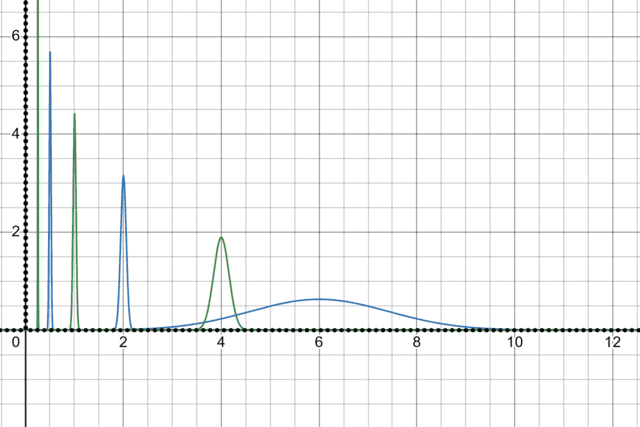
The Dirac delta function is an essential “function” in advanced calculus and physics (particularly, quantum mechanics). A great way to visualize what Dirac delta functions represent is by modeling a mass distribution – Dirac delta functions will exhibit similar behaviors. This means that we observe the behavior of a function at these periods:
狄拉克 δ δδ函数是高等微积分和物理学(尤其是量子力学)中的重要“函数”。要直观理解狄拉克δ δδ函数所代表的含义,一个很好的技巧是对质量分布进行建模——狄拉克δ δδ函数会表现出与之相似的行为。这意味着我们可以借助以下几个阶段观察函数的行为:
- starting when it is near zero
从函数值接近 0 时开始观察; - its increase is suddenly drastic, along with a period of an interval, and
在某一区间内,函数值突然急剧上升; - when the increase slows down and eventually reaches back to zero.
随后上升速度放缓,最终回落至 0。
We can represent the Dirac delta function asδ ( x ) \delta(x)δ(x). We placed a quotation on the function since Dirac delta is technically a tool for us to generalize a certain function that satisfies the equation shown below.
狄拉克 δ δδ函数可表示为δ ( x ) \delta(x)δ(x)。我们给“函数”一词加上引号,是因为从工艺层面来讲,狄拉克δ δδ函数是一种用于推广某类满足下述方程的函数的工具。
∫ − ∞ ∞ δ ( x ) f ( x ) x d x = f ( 0 ) \begin{aligned}\int_{-\infty}^{\infty} \delta(x) f(x) \phantom{x}dx &= f(0)\end{aligned}∫−∞∞δ(x)f(x)xdx=f(0)
This relationship remains true as long as we integrate the expression within an interval that contains0 00in between. We can further expand this relationship into a piecewise function and generalize the upper and lower limits as shown below.
只要我们在包含0 00的区间内对该表达式进行积分,上述关系就始终成立。我们可以将此关系进一步扩展为分段函数,并对积分上下限进行推广,如下所示:
∫ k 1 k 2 δ ( x ) = { 1 , x when x ∈ [ k 1 , k 2 ] 0 , when x ∈ [ k 1 , k 2 ] \begin{aligned}\int_{k_1}^{k_2} \delta(x) = \left\{\begin{matrix}1, \phantom{x} \text{ when } x \in [k_1, k_2]\\0, \text{ when } x \cancel{\in } [k_1, k_2]\end{matrix}\right. \end{aligned}∫k1k2δ(x)={1,x when x∈[k1,k2]0, when x∈[k1,k2]
We can also extend this to account for additional factors within the integrand, such asf ( x ) f(x)f(x)and when the domain is shiftedx 0 x_0x0units.
大家还能够对其进行扩展,以考虑被积函数中的其他因子(如f ( x ) f(x)f(x))以及定义域平移x 0 x_0x0个单位的情况:
∫ k 1 k 2 f ( x ) δ ( x – x 0 ) = { f ( x 0 ) , x when x 0 ∈ [ k 1 , k 2 ] 0 , when x 0 ∈ [ k 1 , k 2 ] \begin{aligned}\int_{k_1}^{k_2} f(x)\delta(x – x_0) = \left\{\begin{matrix}f(x_0), \phantom{x} \text{ when } x_0 \in [k_1, k_2]\\0, \text{ when } x_0 \cancel{ \in } [k_1, k_2]\end{matrix}\right. \end{aligned}∫k1k2f(x)δ(x–x0)={f(x0),x when x0∈[k1,k2]0, when x0∈[k1,k2]
Now that we’ve established the definition and conditions needed for the Dirac delta function, let’s go ahead and deepen our understanding by laying out its main properties.
既然我们已经明确了狄拉克δ δδ函数的定义和所需满足的条件,接下来就凭借阐述其主要性质,进一步加深对该函数的理解。
Dirac Delta Function Properties
狄拉克 δ δδ 函数的性质
The Dirac delta function has a wide range of properties that can help you in evaluating integrals, simplifying differential equations, and applying them to model impulse functions, along with other applications. The three main properties that you need to be aware of are shown below.
狄拉克 δ δδ你应该重点掌握的三个关键性质:就是函数具有多种性质,这些性质不仅能帮助你计算积分、简化微分方程,还能用于冲激函数建模等其他应用场景。以下
Property 1:The Dirac delta function,δ ( x – x 0 ) \delta(x – x_0)δ(x–x0)is equal to zero whenx xxis not equal tox 0 x_0x0.
性质 1:当 x ≠ x 0 x \neq x_0x=x0 时,狄拉克 δ δδ 函数 δ ( x – x 0 ) = 0 \delta(x – x_0) = 0δ(x–x0)=0。
δ ( x – x 0 ) = 0 , when x ≠ x 0 \begin{aligned} \delta(x – x_0) = 0 , \text{ when } x \neq x_0\end{aligned}δ(x–x0)=0, when x=x0
Another way to interpret this is that whenx xxis equal tox 0 x_0x0, the Dirac delta function will return an infinite value.
该性质的另一种解读是:当x = x 0 x = x_0x=x0 时,狄拉克 δ δδ函数的取值为无穷大。
δ ( x – x 0 ) = ∞ , when x = x 0 \begin{aligned} \delta(x – x_0) = \infty , \text{ when } x = x_0\end{aligned}δ(x–x0)=∞, when x=x0
The best way to visualize this property of the Dirac delta function is to imagine how light impulses behave: there are instances when we can no longer measure the energy emitted by the light and there are certain distances when we can. On the instances when it is near impossible to measure the energy, we just assume it’s equal to infinite.
要直观理解狄拉克δ δδ函数的这一性质,最好的方法是联想光冲激的行为:在某些情况下,大家无法测量光发射的能量;而在特定距离下,又能够对其进行测量。对于那些几乎无法测量能量的情况,我们就假设其能量值为无穷大。
Property 2:By integrating the Dirac delta function, we can show that the function is equal to1 11within the allowed interval.
性质 2:对狄拉克 δ δδ函数进行积分可知,在允许的区间内,该积分结果等于1 11。
∫ x 0 – ϵ x 0 + ϵ δ ( x – x 0 ) x d x = 1 , when ϵ > 0 \begin{aligned}\int_{x_0 – \epsilon}^{x_0 + \epsilon} \delta(x – x_0) \phantom{x}dx = 1, \text{ when } \epsilon >0\end{aligned}∫x0–ϵx0+ϵδ(x–x0)xdx=1, when ϵ>0
The upper and lower limits,x 0 – ϵ x_0 – \epsilonx0–ϵ and x 0 + ϵ x_0 + \epsilonx0+ϵ, represent the range that coversx xx. In the context of impulse, this is the range you can observe the behavior of the function.
积分上下限 x 0 – ϵ x_0 – \epsilonx0–ϵ 和 x 0 + ϵ x_0 + \epsilonx0+ϵ 代表包含 x xx你能够观察到函数行为的区间。就是的取值范围。在冲激的场景下,这个范围就
∫ − ∞ ∞ δ ( x – x 0 ) x d x = 1 , when ϵ > 0 \begin{aligned}\int_{-\infty}^{\infty} \delta(x – x_0) \phantom{x}dx = 1, \text{ when } \epsilon >0\end{aligned}∫−∞∞δ(x–x0)xdx=1, when ϵ>0
We can extend this property whenϵ > 0 \epsilon >0ϵ>0and asϵ \epsilonϵapproaches infinity.
当 ϵ > 0 \epsilon >0ϵ>0 且 ϵ \epsilonϵ趋近于无穷大时,我们可以对该性质进行推广。
Property 3:We can extend the second property to account for instances when we multiplyδ ( x ) \delta(x)δ(x)with a function,f ( x ) f(x)f(x).
性质 3:我们可以对性质 2 进行扩展,以涵盖δ ( x ) \delta(x)δ(x) 与某一函数 f ( x ) f(x)f(x)相乘的情况。
∫ x 0 – ϵ x 0 + ϵ f ( x ) δ ( x – x 0 ) x d x = f ( x 0 ) , when ϵ > 0 \begin{aligned}\int_{x_0 – \epsilon}^{x_0 + \epsilon} f(x)\delta(x – x_0) \phantom{x}dx = f(x_0), \text{ when } \epsilon >0\end{aligned}∫x0–ϵx0+ϵf(x)δ(x–x0)xdx=f(x0), when ϵ>0
There are instances whenδ ( x ) \delta(x)δ(x)is equal to zero throughout the interval, so we use nonzero functions such asf ( x ) f(x)f(x)evaluated atx 0 x_0x0. These three properties also highlight the significance of Dirac delta functions in normal and probability distributions.
在某些情况下,δ ( x ) \delta(x)δ(x)在整个区间内都等于 0,因此我们会使用非零函数(如在x 0 x_0x0 处取值的 f ( x ) f(x)f(x))来进行相关计算。这三个性质也凸显了狄拉克δ δδ函数在正态分布和概率分布中的主要意义。
From these properties, we can also see how important Dirac delta functions are in advanced statistics, quantum mechanics, and more. Dirac delta function still has a wide range of important properties, but for now, let’s put our focus on applying Dirac delta functions and see how we can use them and Laplace transforms in solving differential equations and initial value problems.
从这些性质中,我们还能发现狄拉克δ δδ函数在高等统计学、量子力学等领域的重要性。狄拉克δ δδ函数还有许多其他重要性质,但目前我们先将重点放在其应用上,看看如何结合狄拉克δ δδ函数和拉普拉斯变换来求解微分方程和初值问题。
How To Use Dirac Delta Function in Differential Equations?
如何在微分方程中使用狄拉克δ δδ 函数?
We can use the Dirac delta function to solve differential equations by connecting our understanding of Dirac delta functions and Laplace transformations. First, let’s establish the general form of the Dirac delta function’s Laplace transform.
通过将狄拉克δ δδ函数的相关知识与拉普拉斯变换相结合,我们可以利用狄拉克δ δδ函数求解微分方程。起初,我们来确定狄拉克δ δδ函数拉普拉斯变换的一般形式:
L { δ ( x – x 0 ) } = ∫ 0 ∞ e − s t δ ( x – x 0 ) x d t = e − a s \begin{aligned}\mathcal{L}\{\delta(x – x_0)\} &= \int_{0}^{\infty} e^{-st} \delta (x – x_0) \phantom{x}dt \\&= e^{-as}\end{aligned}L{δ(x–x0)}=∫0∞e−stδ(x–x0)xdt=e−as
Keep in mind that our conditions for Laplace transforms must be maintained, soa > 0 a >0a>0. Here are some examples on how we can apply this formula and to be consistent with our Laplace transform notations, we’ll uset ttinstead ofx xxinside the Dirac delta function.
必须注意的是,拉普拉斯变换的条件必须满足,即a > 0 a >0a>0。以下是应用该公式的一些示例,为了与拉普拉斯变换的符号表示保持一致,我们在狄拉克δ δδ函数内部启用t tt 而非 x xx:
| L { δ ( t + 6 ) } = L { δ ( t – − 6 ) } = e 6 s \begin{aligned}\mathcal{L}\{\delta(t + 6)\} &= \mathcal{L}\{\delta(t – -6)\}\\&=e^{6s} \end{aligned}L{δ(t+6)}=L{δ(t–−6)}=e6s | L { 3 δ ( t – 4 ) } = 3 L { δ ( t – 4 ) } = 3 e − 4 s \begin{aligned}\mathcal{L}\{3\delta(t – 4)\} &= 3\mathcal{L}\{\delta(t – 4)\}\\&=3e^{-4s} \end{aligned}L{3δ(t–4)}=3L{δ(t–4)}=3e−4s | L { − 2 δ ( t + 8 ) } = − 2 L { δ ( t – − 8 ) } = − 2 e 8 s \begin{aligned}\mathcal{L}\{-2\delta(t +8)\} &= -2\mathcal{L}\{\delta(t – -8)\}\\&=-2e^{8s}\end{aligned}L{−2δ(t+8)}=−2L{δ(t–−8)}=−2e8s |
|---|
Now, combining this with our previous Laplace transform formulas, we can now use these two concepts to solve linear differential equations. Before we work on an example, let us first write down the Laplace transform functions forf ′ ( t ) f^{\prime}(t)f′(t), f ′ ′ ( t ) f^{\prime \prime}(t)f′′(t), and f ( n ) ( t ) f^{(n)}(t)f(n)(t).
如今,将狄拉克δ δδ函数的拉普拉斯变换与我们之前所学的拉普拉斯变换公式相结合,就行利用这两个概念来求解线性微分方程了。在进行示例演算之前,我们先写出f ′ ( t ) f^{\prime}(t)f′(t)、f ′ ′ ( t ) f^{\prime \prime}(t)f′′(t) 和 f ( n ) ( t ) f^{(n)}(t)f(n)(t)的拉普拉斯变换函数:
| f ( t ) \boldsymbol{f(t)}f(t) 表达式 | L { f ( t ) } = F ( s ) \boldsymbol{\mathcal{L}\{f(t)\} = F(s)}L{f(t)}=F(s) 表达式 |
|---|---|
| y ′ \begin{aligned} y^{\prime }\end{aligned}y′ | s F ( s ) – f ( 0 ) , x s > 0 \begin{aligned} sF(s) – f(0), \phantom{x}s > 0\end{aligned}sF(s)–f(0),xs>0 |
| y ′ ′ \begin{aligned} y^{\prime\prime}\end{aligned}y′′ | s 2 F ( s ) – s f ( 0 ) – f ′ ( 0 ) , x s > 0 \begin{aligned} s^2F(s)– sf(0) – f^{\prime}(0), \phantom{x}s > 0\end{aligned}s2F(s)–sf(0)–f′(0),xs>0 |
| y ( n ) \begin{aligned} y^{(n) }\end{aligned}y(n) | s n F ( s ) − s n − 1 f ( 0 ) − s n − 2 f ′ ( 0 ) − ⋯ − s f ( n − 2 ) ( 0 ) − f ( n − 1 ) ( 0 ) , s > 0 \begin{aligned} s^n F(s) - s^{n-1} f(0) - s^{n-2} f'(0) - \cdots - s f^{(n-2)}(0) - f^{(n-1)}(0), \quad s > 0\end{aligned}snF(s)−sn−1f(0)−sn−2f′(0)−⋯−sf(n−2)(0)−f(n−1)(0),s>0 |
Make sure to have your notes on differential equations, Laplace transforms, and the inverse Laplace transforms before heading over to the next section. We’ll show you an example of how we can use these to solve differential equations using Laplace transforms and the Dirac delta function!
在进入下一部分内容之前,请确保你已备好关于微分方程、拉普拉斯变换和拉普拉斯逆变换的笔记。接下来,大家将通过一个示例,向你展示如何利用拉普拉斯变换和狄拉克δ δδ函数求解微分方程!
Example 1 示例 1
Find the solution to the initial value problem,y ′ ′ – 6 y ′ – 16 y = 4 δ ( t – 8 ) y^{\prime \prime} – 6y ^{\prime} – 16y = 4\delta(t – 8)y′′–6y′–16y=4δ(t–8), wherey ( 0 ) = − 4 y(0) = -4y(0)=−4 and y ′ ( 0 ) = 8 y^{\prime}(0) =8y′(0)=8.
求初值问题 y ′ ′ – 6 y ′ – 16 y = 4 δ ( t – 8 ) y^{\prime \prime} – 6y^{\prime} – 16y = 4\delta(t – 8)y′′–6y′–16y=4δ(t–8)的解,其中初始条件为y ( 0 ) = − 4 y(0) = -4y(0)=−4 且 y ′ ( 0 ) = 8 y^{\prime}(0) =8y′(0)=8。
Solution
解答过程
When working with linear differential equations, we’ll need to take the Laplace transform of both sides of the equation. Use the formulas we’ve provided in the section shown above. Substitute they ( 0 ) y(0)y(0) and y ′ ( 0 ) y^{\prime}(0)y′(0)using our initial conditions.
求解线性微分方程时,需对等式两边同时进行拉普拉斯变换。我们将使用上文给出的拉普拉斯变换公式,并代入初始条件y ( 0 ) y(0)y(0) 和 y ′ ( 0 ) y^{\prime}(0)y′(0) 的值:
s 2 F ( s ) − s f ( 0 ) − f ′ ( 0 ) − 6 ( s F ( s ) − f ( 0 ) ) − 16 F ( s ) = 4 e − 8 s ( s 2 − 6 s − 16 ) F ( s ) − s f ( 0 ) − f ′ ( 0 ) + 6 f ( 0 ) = 4 e − 8 s ( s 2 − 6 s − 16 ) F ( s ) − s ( − 4 ) − 8 + 6 ( − 4 ) = 4 e − 8 s ( s 2 − 6 s − 16 ) F ( s ) + 4 s − 8 − 24 = 4 e − 8 s ( s 2 − 6 s − 16 ) F ( s ) + 4 s − 32 = 4 e − 8 s \begin{aligned}s^2F(s) - s f(0) - f^{\prime}(0) - 6\left(sF(s) - f(0)\right) - 16F(s) &= 4e^{-8s} \\ \left(s^2 - 6s - 16\right)F(s) - s f(0) - f^{\prime}(0) + 6f(0) &= 4e^{-8s} \\ \left(s^2 - 6s - 16\right)F(s) - s(-4) - 8 + 6(-4) &= 4e^{-8s} \\ \left(s^2 - 6s - 16\right)F(s) + 4s - 8 - 24 &= 4e^{-8s} \\ \left(s^2 - 6s - 16\right)F(s) + 4s - 32 &= 4e^{-8s}\end{aligned}s2F(s)−sf(0)−f′(0)−6(sF(s)−f(0))−16F(s)(s2−6s−16)F(s)−sf(0)−f′(0)+6f(0)(s2−6s−16)F(s)−s(−4)−8+6(−4)(s2−6s−16)F(s)+4s−8−24(s2−6s−16)F(s)+4s−32=4e−8s=4e−8s=4e−8s=4e−8s=4e−8s
Divide both sides of the equation bys 2 – 6 s − 16 s^2 – 6s -16s2–6s−16and write down the resulting rational expression as decomposed partial fractions.
将等式两边同时除以s 2 – 6 s − 16 s^2 – 6s -16s2–6s−16,并将得到的有理表达式拆分为部分分式:
( s 2 – 6 s – 16 ) F ( s ) = 4 e − 8 s – 4 ( s – 8 ) F ( s ) = 4 e − 8 s ( s – 2 ) ( s + 8 ) – 4 ( s – 8 ) ( s – 2 ) ( s + 8 ) = 4 e − 8 s G ( s ) – H ( s ) \begin{aligned}(s^2 – 6s – 16)F(s) &= 4e^{-8s} – 4(s – 8)\\ F(s) &= \dfrac{4e^{-8s}}{(s – 2)(s + 8)} – \dfrac{4(s – 8)}{(s – 2)(s + 8)}\\ &= 4e^{-8s} G(s) – H(s)\end{aligned}(s2–6s–16)F(s)F(s)=4e−8s–4(s–8)=(s–2)(s+8)4e−8s–(s–2)(s+8)4(s–8)=4e−8sG(s)–H(s)
其中,G ( s ) = 1 ( s – 2 ) ( s + 8 ) G(s) = \dfrac{1}{(s – 2)(s + 8)}G(s)=(s–2)(s+8)1,H ( s ) = 4 ( s – 8 ) ( s – 2 ) ( s + 8 ) H(s) = \dfrac{4(s – 8)}{(s – 2)(s + 8)}H(s)=(s–2)(s+8)4(s–8)。
Let’s first evaluate the inverse Laplace transform for G ( s ) = 1 ( s – 2 ) ( s + 8 ) G(s) = \dfrac{1}{(s – 2)(s + 8)}G(s)=(s–2)(s+8)1 and H ( s ) = 4 ( s – 8 ) ( s – 2 ) ( s + 8 ) H(s) = \dfrac{4(s – 8)}{(s – 2)(s +8)}H(s)=(s–2)(s+8)4(s–8). As we have mentioned, this is a presumed knowledge, so do head over to the link in case you need a refresher.
首先求解 G ( s ) = 1 ( s – 2 ) ( s + 8 ) G(s) = \dfrac{1}{(s – 2)(s + 8)}G(s)=(s–2)(s+8)1 和 H ( s ) = 4 ( s – 8 ) ( s – 2 ) ( s + 8 ) H(s) = \dfrac{4(s – 8)}{(s – 2)(s +8)}H(s)=(s–2)(s+8)4(s–8)的拉普拉斯逆变换。
Going back to our two Laplace transform functions, here are the resulting functions if we reverse the process to findg ( t ) g(t)g(t) and h ( t ) h(t)h(t):
对上述两个拉普拉斯变换函数进行逆变换,得到g ( t ) g(t)g(t) 和 h ( t ) h(t)h(t) 如下:
| 拉普拉斯变换与逆变换(G(s)与g(t)) | 拉普拉斯变换与逆变换(H(s)与h(t)) |
|---|---|
| G ( s ) = 1 ( s – 2 ) ( s + 8 ) g ( t ) = L − 1 { G ( s ) } = 1 10 e 2 t − 1 10 e − 8 t \begin{aligned} G(s) &= \dfrac{1}{(s – 2)(s + 8)}\\ g(t) &= \mathcal{L}^{-1}\{G(s)\}\\ &= \dfrac{1}{10}e^{2t} - \dfrac{1}{10}e^{-8t}\end{aligned}G(s)g(t)=(s–2)(s+8)1=L−1{G(s)}=101e2t−101e−8t | H ( s ) = 4 s − 32 ( s – 2 ) ( s + 8 ) h ( t ) = L − 1 { H ( s ) } = − 12 5 e 2 t + 32 5 e − 8 t \begin{aligned} H(s) &= \dfrac{4s - 32}{(s – 2)(s +8)}\\ h(t) &= \mathcal{L}^{-1}\{H(s)\}\\ &= -\dfrac{12}{5}e^{2t} + \dfrac{32}{5}e^{-8t}\end{aligned}H(s)h(t)=(s–2)(s+8)4s−32=L−1{H(s)}=−512e2t+532e−8t |
Before we continue, let us establish the Laplace integral property,∫ 0 t δ ( s – k ) x d s = u ( t – k ) \int_{0}^{t} \delta(s – k) \phantom{x}ds = u(t – k)∫0tδ(s–k)xds=u(t–k). Use this to simplify our particular solution further.
在继续求解前,先明确拉普拉斯积分性质:∫ 0 t δ ( s – k ) x d s = u ( t – k ) \int_{0}^{t} \delta(s – k) \phantom{x}ds = u(t – k)∫0tδ(s–k)xds=u(t–k)(其中 u ( t ) u(t)u(t)为单位阶跃函数)。利用该性质进一步简化特解:
F ( s ) = 4 e − 8 s G ( s ) – H ( s ) f ( t ) = 4 u ( t – 8 ) g ( t – 8 ) – h ( t ) = 4 u ( t – 8 ) ⋅ ( 1 10 e 2 ( t – 8 ) − 1 10 e − 8 ( t – 8 ) ) – ( − 12 5 e 2 t + 32 5 e − 8 t ) = 2 5 u ( t – 8 ) ( e 2 t – 16 − e − 8 t + 64 ) + 12 5 e 2 t − 32 5 e − 8 t \begin{aligned}F(s)&= 4e^{-8s} G(s) – H(s)\\ f(t) &= 4u(t – 8)g(t – 8) – h(t)\\ &= 4u(t – 8) \cdot \left( \dfrac{1}{10}e^{2(t – 8)} - \dfrac{1}{10}e^{-8(t – 8)} \right) – \left( -\dfrac{12}{5}e^{2t} + \dfrac{32}{5}e^{-8t} \right)\\ &= \dfrac{2}{5}u(t – 8)\left(e^{2t – 16} - e^{-8t + 64}\right) + \dfrac{12}{5}e^{2t} - \dfrac{32}{5}e^{-8t}\end{aligned}F(s)f(t)=4e−8sG(s)–H(s)=4u(t–8)g(t–8)–h(t)=4u(t–8)⋅(101e2(t–8)−101e−8(t–8))–(−512e2t+532e−8t)=52u(t–8)(e2t–16−e−8t+64)+512e2t−532e−8t
This example shows you how helpful Dirac delta function and Laplace transforms are when finding the particular solution for more complex functions.
该示例表明,在求解复杂函数的特解时,狄拉克δ δδ函数与拉普拉斯变换的结合具有显著作用。
Practice Questions
练习题
Find the Laplace transform of the following Dirac delta functions:
求下列狄拉克δ δδ函数的拉普拉斯变换:
a. δ ( t + 4 ) \delta(t + 4)δ(t+4)
b. 6 δ ( t − 2 ) 6\delta(t -2 )6δ(t−2)
c. − 3 δ ( t + 8 ) -3\delta(t + 8 )−3δ(t+8)Find the solution to the initial value problem,− 2 y ′ ′ – 4 y ′ + 30 y = − 12 δ ( t – 9 ) -2y^{\prime \prime} – 4y^{\prime} +30y = -12\delta(t – 9)−2y′′–4y′+30y=−12δ(t–9), wherey ( 0 ) = − 5 y(0) = -5y(0)=−5 and y ′ ( 0 ) = 7 y^{\prime}(0) =7y′(0)=7.
求初值问题 − 2 y ′ ′ – 4 y ′ + 30 y = − 12 δ ( t – 9 ) -2y^{\prime \prime} – 4y^{\prime} + 30y = -12\delta(t – 9)−2y′′–4y′+30y=−12δ(t–9)的解,其中初始条件为y ( 0 ) = − 5 y(0) = -5y(0)=−5 且 y ′ ( 0 ) = 7 y^{\prime}(0) =7y′(0)=7。Find the solution to the initial value problem,3 y ′ ′ – 9 y ′ + 6 y = 6 δ ( t – 3 ) 3y^{\prime \prime} – 9y^{\prime} +6y = 6\delta(t – 3)3y′′–9y′+6y=6δ(t–3), wherey ( 0 ) = 1 y(0) = 1y(0)=1 and y ′ ( 0 ) = 3 y^{\prime}(0) =3y′(0)=3.
求初值问题 3 y ′ ′ – 9 y ′ + 6 y = 6 δ ( t – 3 ) 3y^{\prime \prime} – 9y^{\prime} + 6y = 6\delta(t – 3)3y′′–9y′+6y=6δ(t–3)的解,其中初始条件为y ( 0 ) = 1 y(0) = 1y(0)=1 且 y ′ ( 0 ) = 3 y^{\prime}(0) =3y′(0)=3。
Answer Key
a. e 4 s e^{4s}e4s
b. 6 e − 2 s 6e^{-2s}6e−2s
c. − 3 e 8 s -3e^{8s}−3e8sy = 3 4 u ( t – 9 ) ( e 3 ( t – 9 ) − e − 5 ( t – 9 ) ) + 1 4 ( − 9 e 3 t + 11 e − 5 t ) y = \dfrac{3}{4}u(t – 9)\left(e^{3(t – 9)} - e^{-5(t – 9)}\right) + \dfrac{1}{4}\left(-9e^{3t} + 11e^{-5t}\right)y=43u(t–9)(e3(t–9)−e−5(t–9))+41(−9e3t+11e−5t)
先对等式两边除以− 2 -2−2简化方程,再利用拉普拉斯变换时移性质求解。
y = u ( t – 3 ) ( e 2 ( t – 3 ) − e t – 3 ) + e 2 t y = u(t – 3)\left(e^{2(t – 3)} - e^{t – 3}\right) + e^{2t}y=u(t–3)(e2(t–3)−et–3)+e2t
方程两边除以3 33后,凭借部分分式分解及逆变换,结合初始条件可消去冗余的− e t -e^t−et 项。
via:
What Exactly is Dirac’s Delta Function?
https://www.physicsforums.com/insights/what-exactly-is-diracs-delta-function/Dirac Delta Function - Definition, Form, and Applications
https://www.storyofmathematics.com/dirac-delta-function/

 浙公网安备 33010602011771号