10.RNN 经典案例:基于 seq2seq 模型的英译法任务实现
学习目标
- 深入理解 seq2seq 模型架构和翻译数据集的特点
- 掌握使用基于 GRU 的 seq2seq 模型实现翻译的完整流程
- 理解并实现解码器端的 Attention 机制
- 学会模型的训练、评估及 Attention 效果可视化分析
一、seq2seq 模型架构详解
1.1 模型整体结构
seq2seq(Sequence to Sequence)模型是一种专门用于处理序列转换任务的神经网络架构,主要由两部分组成:编码器(Encoder) 和解码器(Decoder)。
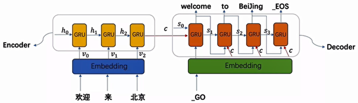
- 编码器:负责处理输入序列(如中文 “欢迎来北京”),通过 GRU 等循环神经网络将整个序列信息压缩成一个中间语义张量
c - 解码器:以中间语义张量
c为输入,逐步生成目标序列(如英文 “welcome to Beijing”)
1.2 模型工作流程
- 输入序列经过嵌入层(Embedding)转换为向量表示
- 编码器 GRU 逐词处理输入序列,输出每个时间步的隐藏状态
- 这些隐藏状态被整合为中间语义张量
c - 解码器 GRU 利用
c和自身隐藏状态,逐词生成目标序列 - 每个生成的词都会作为下一时间步的输入(训练时可使用 teacher forcing 技巧)
1.3 数据集下载
翻译数据集可从 PyTorch 官方教程地址下载:
https://download.pytorch.org/tutorial/data.zip数据集部分预览:
We lost.	Nous avons été défaites.
We lost.	Nous avons été battus.
We lost.	Nous avons été battues.
Who won?	Qui a gagné ?
Who won?	Qui l'a emporté ?
You run.	Tu cours.
Am I fat?	Suis-je gros ?
Am I fat?	Suis-je grosse ?
Back off.	Recule !
Back off.	Reculez.
Back off.	Retire-toi !
从上面数据格式可以看出,每一行都是一对英语和法语的相同意思的数据,并且两种语言的数据通过制表符“\t”分割
二、数据预处理
2.1工具包与环境
import torch
import torch.nn as nn
import torch.optim as optim
from torch.utils.data import Dataset, DataLoader, random_split
import numpy as np
import re  # 正则表达式处理文本
import matplotlib.pyplot as plt
import seaborn as sns  # 更美观的可视化
from tqdm import tqdm  # 训练进度条
import unicodedata  # 处理特殊字符
import random#用于随机生成数据
import torch.nn.functional as F
import time

# 设置随机种子确保结果可复现
torch.manual_seed(42)
np.random.seed(42)

# 检查GPU加速是否可用
device = torch.device("cuda" if torch.cuda.is_available() else "cpu")
print(f"使用的计算设备: {device}")
2.2 数据预处理工具类
2.2.1 语言映射类(Lang)
该类用于将词汇与数值索引进行双向映射,是自然语言处理中的基础操作。
# 句子开始标志
SOS_token = 0
# 句子结束标志
EOS_token = 1

class Lang:
    def __init__(self, name):
        """初始化语言对象
        参数:
            name: 语言名称(如'eng'表示英语,'fra'表示法语)
        """
        self.name = name
        self.word2index = {}  # 词汇到索引的映射字典
        self.index2word = {SOS_token: "SOS", EOS_token: "EOS"}  # 索引到词汇的映射字典
        self.n_words = 2  # 词汇总数,初始为2(SOS和EOS已占用)

    def addWord(self, word):
        """添加词汇到映射表
        参数:
            word: 要添加的词汇
        """
        # 如果词汇不在映射表中,则添加它
        if word not in self.word2index:
            self.word2index[word] = self.n_words
            self.index2word[self.n_words] = word
            self.n_words += 1  # 词汇计数加1

    def addSentence(self, sentence):
        """将句子拆分为词汇并添加到映射表
        参数:
            sentence: 要处理的句子
        """
        # 按空格分割句子为词汇列表
        for word in sentence.split(' '):
self.addWord(word)使用示例:
# 创建英语语言对象
eng = Lang('eng')
# 添加句子到语言对象
eng.addSentence("hello I am Jay")

print("词汇到索引映射:", eng.word2index)  # {'hello': 2, 'I': 3, 'am': 4, 'Jay': 5}
print("索引到词汇映射:", eng.index2word)  # {0: 'SOS', 1: 'EOS', 2: 'hello', 3: 'I', 4: 'am', 5: 'Jay'}
print("词汇总数:", eng.n_words)  # 6
2.2.2 文本规范化函数
用于处理特殊字符、统一格式,提高数据质量。
import unicodedata
import re

def unicodeToAscii(s):
    """将Unicode字符串转换为ASCII字符
    主要用于去除重音标记等特殊符号
    参数:
        s: 待转换的Unicode字符串
    返回:
        转换后的ASCII字符串
    """
    return ''.join(
        c for c in unicodedata.normalize('NFD', s)
        if unicodedata.category(c) != 'Mn'
    )

def normalizeString(s):
    """字符串规范化处理
    参数:
        s: 待规范化的字符串
    返回:
        规范化后的字符串
    """
    # 转为小写并去除首尾空格,再去除重音标记
    s = unicodeToAscii(s.lower().strip())
    # 在标点符号前添加空格,便于后续分割
    s = re.sub(r"([.!?])", r" \1", s)
    # 移除非字母和标点的字符
    s = re.sub(r"[^a-zA-Z.!?]+", r" ", s)
return s使用示例:
s = "Are you kidding me?"
normalized_s = normalizeString(s)
print(normalized_s)  # 输出: "are you kidding me ?"
2.3 数据集加载与过滤
2.3.1 加载语言数据
def readLangs(lang1, lang2, data_path):
    """读取语言数据文件并创建语言对象
    参数:
        lang1: 源语言名称(如'eng')
        lang2: 目标语言名称(如'fra')
        data_path: 数据文件路径
    返回:
        input_lang: 源语言对象
        output_lang: 目标语言对象
        pairs: 语言对列表
    """
    # 读取文件内容并按行分割
    lines = open(data_path, encoding='utf-8').read().strip().split('\n')

    # 对每一行进行分割和规范化处理
    pairs = [[normalizeString(s) for s in l.split('\t')] for l in lines]

    # 创建语言对象
    input_lang = Lang(lang1)
    output_lang = Lang(lang2)

    return input_lang, output_lang, pairs
2.3.2 过滤语言对
为了提高训练效率和效果,我们过滤出符合要求的语言对:
# 句子最大长度限制
MAX_LENGTH = 10

# 选择带有指定前缀的英语句子作为训练数据
eng_prefixes = (
    "we are", "we re ",
    "they are", "they re ",
    "i am", "i m ",
    "you are", "you re ",
    "he is", "she is",
    "it is", "we will",
    "they will", "i will"
)

def filterPair(p):
    """过滤单个语言对
    参数:
        p: 语言对,格式为[源语言句子, 目标语言句子]
    返回:
        布尔值,True表示符合要求,False表示不符合
    """
    # 检查句子长度是否在限制范围内,且源语言句子是否以指定前缀开头
    return len(p[0].split(' ')) < MAX_LENGTH and \
           p[0].startswith(eng_prefixes) and \
           len(p[1].split(' ')) < MAX_LENGTH

def filterPairs(pairs):
    """过滤语言对列表
    参数:
        pairs: 待过滤的语言对列表
    返回:
        过滤后的语言对列表
    """
    return [pair for pair in pairs if filterPair(pair)]
2.3.3 数据准备整合函数
def prepareData(lang1, lang2, data_path):
    """数据准备主函数
    完成从文件读取到数据过滤、词汇映射的全过程
    参数:
        lang1: 源语言名称
        lang2: 目标语言名称
        data_path: 数据文件路径
    返回:
        input_lang: 源语言对象
        output_lang: 目标语言对象
        pairs: 过滤后的语言对列表
    """
    # 读取语言数据
    input_lang, output_lang, pairs = readLangs(lang1, lang2, data_path)
    print(f"读取原始语言对数量: {len(pairs)}")

    # 过滤语言对
    pairs = filterPairs(pairs)
    print(f"过滤后语言对数量: {len(pairs)}")

    # 构建词汇表
    for pair in pairs:
        input_lang.addSentence(pair[0])
        output_lang.addSentence(pair[1])

    print(f"源语言词汇总数: {input_lang.n_words}")
    print(f"目标语言词汇总数: {output_lang.n_words}")

return input_lang, output_lang, pairs使用示例:
# 数据文件路径(请替换为实际路径)
data_path = "D:/learn/000人工智能数据大全/nlp/NLP基础课所有数据和代码/eng-fra.txt"

# 准备数据
input_lang, output_lang, pairs = prepareData('eng', 'fra', data_path)

# 打印示例
print("随机示例语言对:", random.choice(pairs))
读取原始语言对数量: 135842
过滤后语言对数量: 10275
源语言词汇总数: 2742
目标语言词汇总数: 4355
随机示例语言对: ['i am lazy .', 'je suis faineant .']2.4 数据转换为张量
将文本数据转换为模型可接受的张量形式:
import torch

def tensorFromSentence(lang, sentence):
    """将句子转换为张量
    参数:
        lang: 语言对象
        sentence: 待转换的句子
    返回:
        句子对应的张量
    """
    # 将句子分割为词汇并转换为索引
    indexes = [lang.word2index[word] for word in sentence.split(' ')]
    # 添加句子结束标志
    indexes.append(EOS_token)
    # 转换为张量并调整形状
    return torch.tensor(indexes, dtype=torch.long, device=device).view(-1, 1)

def tensorsFromPair(pair, input_lang, output_lang):
    """将语言对转换为张量对
    参数:
        pair: 语言对
        input_lang: 源语言对象
        output_lang: 目标语言对象
    返回:
        源语言张量和目标语言张量组成的元组
    """
    input_tensor = tensorFromSentence(input_lang, pair[0])
    target_tensor = tensorFromSentence(output_lang, pair[1])
    return (input_tensor, target_tensor)
调用示例:
pare=pairs[0]
input_tensor, target_tensor=tensorsFromPair(pare, input_lang, output_lang)
print('input_tensor:\n',input_tensor)
print('target_tensor:\n',target_tensor)
input_tensor:
tensor([[2],
[3],
[4],
[1]])
target_tensor:
tensor([[2],
[3],
[4],
[5],
[1]])三、构建基于 GRU 的 seq2seq 模型
3.1 编码器(Encoder)实现
编码器结构图:
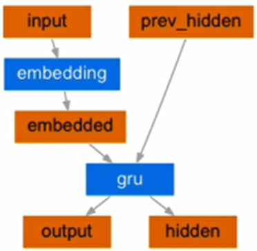
编码器的作用是将输入序列转换为中间语义表示,使用 GRU 作为核心网络结构。
import torch.nn as nn
import torch.nn.functional as F

class EncoderRNN(nn.Module):
    def __init__(self, input_size, hidden_size, device):
        """初始化编码器
        参数:
            input_size: 输入词汇表大小
            hidden_size: 隐藏层大小(同时也是词嵌入维度)
            device: 运行设备(CPU或GPU)
        """
        super(EncoderRNN, self).__init__()
        self.hidden_size = hidden_size
        self.device = device

        # 词嵌入层:将词汇索引转换为向量表示
        self.embedding = nn.Embedding(input_size, hidden_size)
        # GRU层:处理序列信息
        self.gru = nn.GRU(hidden_size, hidden_size)

    def forward(self, input, hidden):
        """前向传播
        参数:
            input: 输入张量,形状为(1, 1)
            hidden: 隐藏状态张量,形状为(1, 1, hidden_size)
        返回:
            output: GRU输出,形状为(1, 1, hidden_size)
            hidden: 更新后的隐藏状态,形状为(1, 1, hidden_size)
        """
        # 词嵌入并调整形状为(1, 1, hidden_size)
        embedded = self.embedding(input).view(1, 1, -1)
        output = embedded
        # 通过GRU处理
        output, hidden = self.gru(output, hidden)
        return output, hidden

    def initHidden(self):
        """初始化隐藏状态
        返回:
            初始化的隐藏状态张量,全为0
        """
        return torch.zeros(1, 1, self.hidden_size, device=self.device)
input_size定义了词嵌入层的输入维度,即词汇表中不同词的数量。- 它决定了嵌入矩阵的行数(例如,
input_size=100表示嵌入矩阵有 100 行,每行对应一个词)。- 如果你的词汇表实际有 5000 个词,但设置
input_size=100,会导致索引超出范围错误,因为模型无法表示词汇表中索引大于 99 的词。
view(1, 1, -1)是为了适配 GRU 的输入格式,与input_size无关。- GRU 要求输入形状为
(seq_len, batch_size, hidden_size),这里:
seq_len=1(每次处理 1 个词)batch_size=1(每次处理 1 个样本)hidden_size是词向量的维度(由nn.Embedding的第二个参数决定)嵌入矩阵的行数=
input_size,大小等于词汇表的大小;嵌入矩阵的列数=
hidden_size,大小意味着每个词被表示成多少维。示例说明
假设:
input_size=100,表示词汇表有 100 个词(索引 0~99)。hidden_size=25,表示每个词被编码为 25 维的向量。当输入一个词的索引(如input=5)时:
self.embedding(input)会从嵌入矩阵中取出第 5 行,得到形状为[25]的向量。.view(1, 1, -1)将其重塑为[1, 1, 25],适配 GRU 的输入。如果词汇表实际有 5000 个词,但你设置input_size=100,当输入索引为 500 的词时,会触发错误IndexError: index out of range in self如何正确设置
input_size?在实际应用中,input_size应等于词汇表的大小。例如,在你的英 - 法翻译任务中:input_lang, output_lang, pairs = prepareData('eng', 'fra', data_path) # input_lang.n_words 是实际词汇表大小 encoder = EncoderRNN(input_lang.n_words, hidden_size, device)这样设置后,模型才能正确处理训练数据中的所有词汇。
测试代码:
hidden_size=25
input_size=100
input=input_tensor[0][0]
rnn_encoder=EncoderRNN(input_size, hidden_size, device)
hidden=rnn_encoder.initHidden()
print('经过GRU之前的hidden:\n', hidden)
output_res,hidden=rnn_encoder(input,hidden)
print('经过GRU之后的output_res:\n', output_res)
print('经过GRU之后的hidden:\n', hidden)
经过GRU之前的hidden:
tensor([[[0., 0., 0., 0., 0., 0., 0., 0., 0., 0., 0., 0., 0., 0., 0., 0., 0., 0., 0., 0., 0., 0., 0.,
0., 0.]]])
经过GRU之后的output_res:
tensor([[[-1.3576e-01, -4.0981e-01, 4.5557e-01, -3.9484e-04, 3.2677e-01,
-1.2381e-02, -2.6698e-01, 4.0892e-01, 1.5625e-01, -1.2065e-01,
1.4958e-01, -5.3734e-01, 1.0011e-03, -3.0357e-01, -6.5508e-02,
-2.5837e-01, 1.5218e-01, 1.6780e-01, 6.3804e-02, 1.8815e-01,
4.2681e-02, -4.5421e-02, -7.1564e-02, 1.1518e-01, 4.7800e-02]]],
grad_fn=<StackBackward0>)
经过GRU之后的hidden:
tensor([[[-1.3576e-01, -4.0981e-01, 4.5557e-01, -3.9484e-04, 3.2677e-01,
-1.2381e-02, -2.6698e-01, 4.0892e-01, 1.5625e-01, -1.2065e-01,
1.4958e-01, -5.3734e-01, 1.0011e-03, -3.0357e-01, -6.5508e-02,
-2.5837e-01, 1.5218e-01, 1.6780e-01, 6.3804e-02, 1.8815e-01,
4.2681e-02, -4.5421e-02, -7.1564e-02, 1.1518e-01, 4.7800e-02]]],
grad_fn=<StackBackward0>)编码器工作原理:
- 输入词汇通过嵌入层转换为向量表示
- 向量输入 GRU 网络,得到输出和更新后的隐藏状态
- 对于整个输入序列,编码器会逐词处理,最终输出的隐藏状态包含了整个序列的信息
3.2 带 Attention 机制的解码器(Decoder)实现
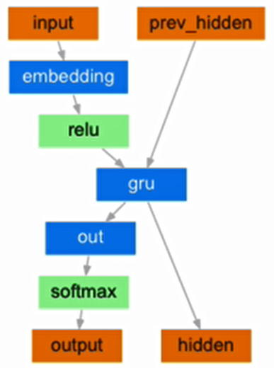
解码器结构图:

解码器负责将编码器生成的中间语义表示转换为目标序列,加入 Attention 机制可以让解码器在生成每个词时关注输入序列的不同部分。
class AttnDecoderRNN(nn.Module):
    def __init__(self, hidden_size, output_size, dropout_p=0.1, max_length=MAX_LENGTH, device=None):
        """初始化带Attention机制的解码器
        参数:
            hidden_size: 隐藏层大小(与编码器保持一致)
            output_size: 输出词汇表大小
            dropout_p: dropout概率,用于防止过拟合
            max_length: 最大句子长度,用于Attention权重计算
            device: 运行设备
        """
        super(AttnDecoderRNN, self).__init__()
        self.hidden_size = hidden_size
        self.output_size = output_size
        self.dropout_p = dropout_p
        self.max_length = max_length
        self.device = device

        # 词嵌入层
        self.embedding = nn.Embedding(self.output_size, self.hidden_size)
        # Attention机制中的线性层,用于计算注意力权重
        self.attn = nn.Linear(self.hidden_size * 2, self.max_length)
        # 整合Attention结果和当前输入的线性层
        self.attn_combine = nn.Linear(self.hidden_size * 2, self.hidden_size)
        # Dropout层
        self.dropout = nn.Dropout(self.dropout_p)
        # GRU层
        self.gru = nn.GRU(self.hidden_size, self.hidden_size)
        # 输出层,将GRU输出映射到词汇表大小
        self.out = nn.Linear(self.hidden_size, self.output_size)

    def forward(self, input, hidden, encoder_outputs):
        """前向传播
        参数:
            input: 输入张量,形状为(1, 1)
            hidden: 隐藏状态张量,形状为(1, 1, hidden_size)
            encoder_outputs: 编码器所有时间步的输出,形状为(max_length, hidden_size)
        返回:
            output: 解码器输出,形状为(1, output_size)
            hidden: 更新后的隐藏状态
            attn_weights: 注意力权重,形状为(1, max_length)
        """
        # 词嵌入并调整形状
        embedded = self.embedding(input).view(1, 1, -1)
        # 应用dropout防止过拟合
        embedded = self.dropout(embedded)

        # 计算注意力权重
        attn_weights = F.softmax(
            self.attn(torch.cat((embedded[0], hidden[0]), 1)), dim=1)

        # 应用注意力权重到编码器输出
        attn_applied = torch.bmm(attn_weights.unsqueeze(0),
                                 encoder_outputs.unsqueeze(0))

        # 整合注意力结果和当前输入
        output = torch.cat((embedded[0], attn_applied[0]), 1)
        output = self.attn_combine(output).unsqueeze(0)

        # 激活函数处理
        output = F.relu(output)
        # GRU处理
        output, hidden = self.gru(output, hidden)

        # 输出层处理并应用log softmax
        output = F.log_softmax(self.out(output[0]), dim=1)
        return output, hidden, attn_weights

    def initHidden(self):
        """初始化隐藏状态
        返回:
            初始化的隐藏状态张量,全为0
        """
        return torch.zeros(1, 1, self.hidden_size, device=self.device)
Attention 机制工作原理:
- 计算解码器当前状态与编码器每个时间步输出的相关性(注意力权重)
- 根据注意力权重对编码器输出进行加权求和
- 将加权结果与当前输入结合,作为 GRU 的输入
- 这样解码器在生成每个词时,会更加关注输入序列中相关的部分
四、模型训练
4.1 训练函数实现
什么是teacher_forcing?
它是一种用于序列生成任务的训练技巧,在seq2seq架构中,根据循环神经网络理论,解码器每次应该使用上一步的结果作为输入的一部分,但是训练过程中,一旦上一步的结果是错误的,就会导致这种错误被累积,无法达到训练效果,因此,我们需要一种机制改变上一步出错的情况,因为训练时我们是已知正确的输出应该是什么,因此可以强制将上一步结果设置成正确的输出,这种方式就叫做teacher_forcing。
teacher_forcing的作用:
能够在训练的时候矫正模型的预测,避免在序列生成的过程中误差进一步放大teacher_forcing能够极大的加快模型的收敛速度,令模型训练过程更快更平稳。
构建训练函数:
# 设置teacher_forcing比率为0.5
teacher_forcing_ratio=0.5
def train(input_tensor, target_tensor, encoder, decoder,
          encoder_optimizer, decoder_optimizer, criterion,
          max_length=MAX_LENGTH, device=None):
    """训练单个样本
    参数:
        input_tensor: 输入序列张量
        target_tensor: 目标序列张量
        encoder: 编码器模型
        decoder: 解码器模型
        encoder_optimizer: 编码器优化器
        decoder_optimizer: 解码器优化器
        criterion: 损失函数
        max_length: 最大句子长度
        device: 运行设备
    返回:
        平均损失值
    """
    # 初始化编码器隐藏状态
    encoder_hidden = encoder.initHidden()

    # 梯度清零
    encoder_optimizer.zero_grad()
    decoder_optimizer.zero_grad()

    # 获取输入和目标序列长度
    input_length = input_tensor.size(0)
    target_length = target_tensor.size(0)

    # 初始化编码器输出存储张量
    encoder_outputs = torch.zeros(max_length, encoder.hidden_size, device=device)

    loss = 0  # 初始化损失

    # 编码器处理输入序列
    for ei in range(input_length):
        encoder_output, encoder_hidden = encoder(
            input_tensor[ei], encoder_hidden)
        encoder_outputs[ei] = encoder_output[0, 0]

    # 解码器初始输入为SOS_token
    decoder_input = torch.tensor([[SOS_token]], device=device)

    # 解码器初始隐藏状态为编码器最后一个隐藏状态
    decoder_hidden = encoder_hidden

    # 随机决定是否使用teacher forcing
    use_teacher_forcing = True if random.random() < teacher_forcing_ratio else False

    if use_teacher_forcing:
        # Teacher forcing: 直接使用目标序列作为解码器输入
        for di in range(target_length):
            decoder_output, decoder_hidden, decoder_attention = decoder(
                decoder_input, decoder_hidden, encoder_outputs)
            loss += criterion(decoder_output, target_tensor[di])
            decoder_input = target_tensor[di]  # 下一个输入是目标序列的下一个词

    else:
        # 不使用teacher forcing: 使用解码器自身输出作为下一个输入
        for di in range(target_length):
            decoder_output, decoder_hidden, decoder_attention = decoder(
                decoder_input, decoder_hidden, encoder_outputs)
            topv, topi = decoder_output.topk(1)
            decoder_input = topi.squeeze().detach()  # 从输出中选择概率最高的词作为下一个输入

            loss += criterion(decoder_output, target_tensor[di])
            if decoder_input.item() == EOS_token:
                break  # 如果生成了结束标志,则提前结束

    # 反向传播计算梯度
    loss.backward()

    # 更新编码器和解码器参数
    encoder_optimizer.step()
    decoder_optimizer.step()

    # 返回平均损失
    return loss.item() / target_length
4.2 训练辅助函数
4.2.1 时间计算函数
用于跟踪训练耗时:
def timeSince(since):
    """计算从某个时间点到现在的耗时
    参数:
        since: 起始时间戳
    返回:
        格式化的时间字符串(分:秒)
    """
    now = time.time()
    s = now - since
    m = math.floor(s / 60)
    s -= m * 60
    return '%dm %ds' % (m, s)
4.2.2 训练迭代函数
import matplotlib.pyplot as plt
import matplotlib.font_manager as fm

# 设置中文字体
plt.rcParams["font.family"] = ["SimHei", "WenQuanYi Micro Hei", "Heiti TC"]
plt.rcParams['axes.unicode_minus'] = False  # 解决负号显示问题

def trainIters(encoder, decoder, n_iters, print_every=1000, plot_every=100, learning_rate=0.01):
    """模型训练主函数
    参数:
        encoder: 编码器模型
        decoder: 解码器模型
        n_iters: 训练迭代次数
        print_every: 每隔多少迭代打印一次训练信息
        plot_every: 每隔多少迭代记录一次损失用于绘图
        learning_rate: 学习率
    """
    start = time.time()  # 记录开始时间
    plot_losses = []  # 用于存储绘图用的损失值
    print_loss_total = 0  # 打印间隔内的总损失
    plot_loss_total = 0  # 绘图间隔内的总损失

    # 定义优化器
    encoder_optimizer = optim.SGD(encoder.parameters(), lr=learning_rate)
    decoder_optimizer = optim.SGD(decoder.parameters(), lr=learning_rate)

    # 随机选择训练样本
    training_pairs = [tensorsFromPair(random.choice(pairs), input_lang, output_lang)
                      for i in range(n_iters)]

    # 定义损失函数(负对数似然损失)
    criterion = nn.NLLLoss()

    # 开始迭代训练
    for iter in range(1, n_iters + 1):
        training_pair = training_pairs[iter - 1]
        input_tensor = training_pair[0]
        target_tensor = training_pair[1]

        # 进行一次训练并计算损失
        loss = train(input_tensor, target_tensor, encoder,
                     decoder, encoder_optimizer, decoder_optimizer, criterion)
        print_loss_total += loss
        plot_loss_total += loss

        # 打印训练信息
        if iter % print_every == 0:
            print_loss_avg = print_loss_total / print_every
            print_loss_total = 0
            print('%s (%d %d%%) %.4f' % (timeSince(start),
                                         iter, iter / n_iters * 100, print_loss_avg))

        # 记录绘图用的损失
        if iter % plot_every == 0:
            plot_loss_avg = plot_loss_total / plot_every
            plot_losses.append(plot_loss_avg)
            plot_loss_total = 0

    # 绘制损失曲线
    plt.figure(figsize=(10, 6))
    plt.plot(plot_losses)
    plt.xlabel('迭代次数(×{})'.format(plot_every))
    plt.ylabel('损失值')
    plt.title('训练损失曲线')
    plt.savefig('training_loss.png')
    plt.show()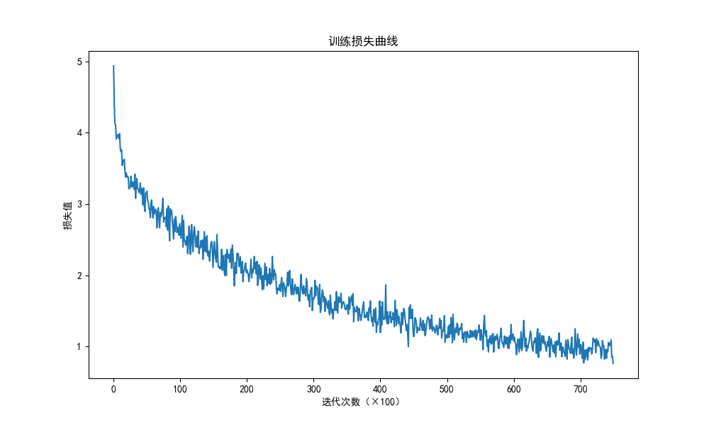
损失曲线分析:
一直下降的损失曲线,说明模型正在收敛,能够从数据中找到一些规律应用于数据
4.3 模型训练过程
# 设置设备(优先使用GPU)
device = torch.device("cuda" if torch.cuda.is_available() else "cpu")

# 模型参数设置
hidden_size = 256  # 隐藏层大小
teacher_forcing_ratio = 0.5  # teacher forcing比例

# 实例化编码器和解码器
encoder = EncoderRNN(input_lang.n_words, hidden_size, device).to(device)
decoder = AttnDecoderRNN(hidden_size, output_lang.n_words, dropout_p=0.1, device=device).to(device)

# 开始训练
print("开始训练...")
trainIters(encoder, decoder, 75000, print_every=5000)训练过程说明:
- 训练迭代次数设为 75000 次,每 5000 次打印一次训练信息
- 采用随机梯度下降(SGD)作为优化器
- 损失函数使用负对数似然损失(NLLLoss),适合分类任务
- 训练过程中会自动记录损失并绘制损失曲线,便于观察模型收敛情况
点击查看打印结果
开始训练...
3m 26s (5000 6%) 3.4770
6m 56s (10000 13%) 2.8251
10m 26s (15000 20%) 2.4605
13m 58s (20000 26%) 2.1898
17m 31s (25000 33%) 1.9971
21m 4s (30000 40%) 1.8023
24m 38s (35000 46%) 1.6236
28m 12s (40000 53%) 1.4830
31m 46s (45000 60%) 1.3988
35m 19s (50000 66%) 1.2732
38m 53s (55000 73%) 1.2022
42m 28s (60000 80%) 1.1113
46m 2s (65000 86%) 1.0620
49m 37s (70000 93%) 0.9985
53m 12s (75000 100%) 0.9625
五、模型评估与测试
5.1 评估函数实现
def evaluate(encoder, decoder, sentence, max_length=MAX_LENGTH):
    """模型评估函数
    参数:
        encoder: 训练好的编码器
        decoder: 训练好的解码器
        sentence: 待评估的句子
        max_length: 最大序列长度
    返回:
        output_words: 生成的目标序列词汇列表
        attentions: 注意力权重矩阵
    """
    with torch.no_grad():  # 评估时不计算梯度
        # 将输入句子转换为张量
        input_tensor = tensorFromSentence(input_lang, sentence)
        input_length = input_tensor.size()[0]
        encoder_hidden = encoder.initHidden()

        # 初始化编码器输出存储张量
        encoder_outputs = torch.zeros(max_length, encoder.hidden_size, device=device)

        # 编码器处理输入句子
        for ei in range(input_length):
            encoder_output, encoder_hidden = encoder(input_tensor[ei],
                                                     encoder_hidden)
            encoder_outputs[ei] += encoder_output[0, 0]

        # 解码器初始输入为SOS_token
        decoder_input = torch.tensor([[SOS_token]], device=device)
        decoder_hidden = encoder_hidden  # 解码器初始隐藏状态为编码器最后一个隐藏状态

        output_words = []  # 存储生成的词汇
        decoder_attentions = torch.zeros(max_length, max_length)  # 存储注意力权重

        # 解码器生成目标序列
        for di in range(max_length):
            decoder_output, decoder_hidden, decoder_attention = decoder(
                decoder_input, decoder_hidden, encoder_outputs)
            decoder_attentions[di] = decoder_attention.data  # 记录注意力权重

            # 选择概率最高的词汇
            topv, topi = decoder_output.data.topk(1)
            if topi.item() == EOS_token:
                output_words.append('<EOS>')  # 遇到结束标志则停止
                break
            else:
                output_words.append(output_lang.index2word[topi.item()])

            decoder_input = topi.squeeze().detach()  # 更新解码器输入

        return output_words, decoder_attentions[:di + 1]
5.2 随机测试函数
def evaluateRandomly(encoder, decoder, n=10):
    """随机测试函数,用于直观展示模型翻译效果
    参数:
        encoder: 训练好的编码器
        decoder: 训练好的解码器
        n: 测试样本数量
    """
    for i in range(n):
        pair = random.choice(pairs)  # 随机选择一个语言对
        print('>', pair[0])  # 输入句子
        print('=', pair[1])  # 正确翻译结果

        # 模型预测
        output_words, attentions = evaluate(encoder, decoder, pair[0])
        output_sentence = ' '.join(output_words)
        print('<', output_sentence)  # 模型输出结果
        print('')  # 空行分隔
5.3 模型测试与结果分析
# 进行随机测试
print("开始随机测试...")
evaluateRandomly(encoder, decoder)测试结果示例:
点击查看随机测试结果
开始随机测试...
> i m sure that tom will do that .
= je suis sure que tom va le faire .
< je suis sure que tom va le faire . <EOS>

> you aren t invited .
= tu n es pas invitee .
< vous n etes pas invite . <EOS>

> i am too tired to climb .
= je suis trop fatigue pour grimper .
< je suis trop fatigue pour continuer . <EOS>

> i m friends with all those guys .
= je suis ami avec tous ces gars la .
< je suis ami avec tous les gars . <EOS>

> i am no match for him .
= je ne peux pas me comparer a lui .
< je ne suis pas lui lui non . <EOS>

> we re changing it .
= nous sommes en train de le changer .
< nous sommes en train de le changer . <EOS>

> i m contented .
= me voila satisfait .
< me voila . <EOS>

> i am alarmed by your irresponsible attitude .
= je suis inquiet de votre attitude irresponsable .
< je suis etonne par ton attitude irresponsable . <EOS>

> they re mine .
= elles sont miennes .
< elles sont a moi . <EOS>

> it is impossible for you to succeed .
= il vous est impossible de reussir .
< il est impossible pour reussir . <EOS>

输入: we are both teachers .
输出: nous sommes tous deux enseignants enseignants . <EOS>结果分析:
- 模型对大部分句子能够生成正确或接近正确的翻译
- 部分句子存在语法或用词错误(如 "she is beautiful like her mother" 的翻译)
- 性别一致问题在法语翻译中仍有不足(如 "impressionne" 和 "impressionnee" 的性别差异)
- 整体来看,模型已经学习到了基本的英法翻译规律,但在复杂句式和细节上仍有提升空间
5.4 Attention 机制可视化
import matplotlib.ticker as ticker
import matplotlib.pyplot as plt
import matplotlib.font_manager as fm

# 设置中文字体
plt.rcParams["font.family"] = ["SimHei", "WenQuanYi Micro Hei", "Heiti TC"]
plt.rcParams['axes.unicode_minus'] = False  # 解决负号显示问题

def showAttention(input_sentence, output_words, attentions):
    """可视化Attention权重
    参数:
        input_sentence: 输入句子
        output_words: 输出词汇列表
        attentions: 注意力权重矩阵
    """
    # 设置图形大小
    fig = plt.figure(figsize=(10, 8))
    ax = fig.add_subplot(111)

    # 绘制注意力热图
    cax = ax.matshow(attentions.numpy(), cmap='bone')
    fig.colorbar(cax)

    # 设置坐标轴刻度
    ax.xaxis.set_major_locator(ticker.MultipleLocator(1))
    ax.yaxis.set_major_locator(ticker.MultipleLocator(1))

    # 设置坐标轴标签
    ax.set_xticklabels([''] + input_sentence.split(' ') + ['<EOS>'], rotation=90)
    ax.set_yticklabels([''] + output_words)

    plt.show()

def evaluateAndShowAttention(input_sentence):
    """评估并可视化注意力权重
    参数:
        input_sentence: 输入句子
    """
    output_words, attentions = evaluate(encoder, decoder, input_sentence)
    print('输入:', input_sentence)
    print('输出:', ' '.join(output_words))
    showAttention(input_sentence, output_words, attentions)

# 可视化特定句子的注意力权重
evaluateAndShowAttention("we are both teachers .")使用示例:
# 可视化特定句子的注意力权重
evaluateAndShowAttention("we are both teachers .")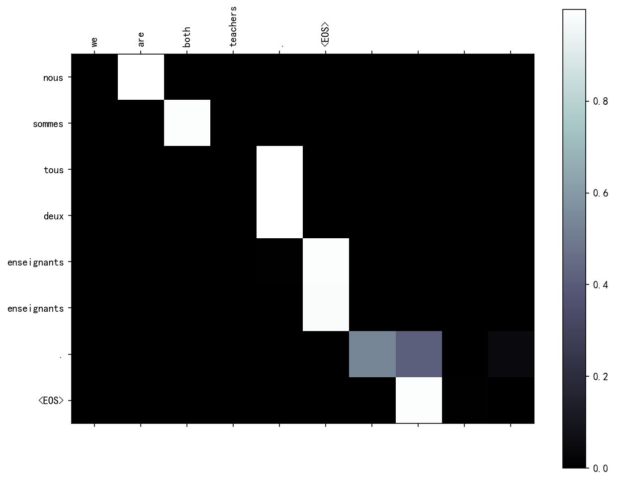
分析:
Attention图像的纵坐标代表输入的源语言各个词汇对应的索引,0-6分别对应["we”,"re”"both",“teachers","",”],纵坐标代表生成的目标语言各个词汇对应的索引,0-7代表['nous','sommes','toutes','deux,'enseignantes,…”,图中浅色小方块(颜色越浅说明影响越大)代表词汇之间的影响关系,比如源语言的第1个词汇对生成目标语言的第1个词汇影响最大,源语言的第4,5个词对生成目标语言的第5个词会影响最大,通过这样的可视化图像,我们可以知道Attention的效果好坏,与我们人为去判定到底还有多大的差距.进而衡量我们训练模型的可用性
Attention 可视化结果分析:
- 热力图的横坐标表示输入句子的词汇
- 纵坐标表示生成的目标句子的词汇
- 颜色越深表示注意力权重越大,说明生成对应目标词汇时,模型更关注输入句子中的该词汇
- 通过注意力可视化,可以直观地看到模型在翻译过程中关注的重点,有助于理解模型的决策过程
六、总结与扩展
6.1 本教程总结
本教程详细介绍了使用基于 GRU 的 seq2seq 模型实现英译法任务的全过程,主要包括:
- 模型架构:seq2seq 模型由编码器和解码器两部分组成,分别负责输入序列的编码和目标序列的生成
- 数据处理:包括文本规范化、词汇映射、张量转换等步骤,将原始文本数据转换为模型可接受的格式
- 模型实现:实现了基于 GRU 的编码器和带 Attention 机制的解码器,Attention 机制能帮助模型更好地关注输入序列的相关部分
- 模型训练:使用随机梯度下降优化器和负对数似然损失函数进行训练,引入 teacher forcing 技巧加速收敛
- 模型评估:实现了评估函数和随机测试函数,通过可视化 Attention 权重分析模型的翻译过程
6.2 可能的改进方向
- 使用更先进的网络结构:如 LSTM 替代 GRU,或使用 Transformer 模型(目前主流的翻译模型)
- 增加训练数据量:更大的数据集通常能带来更好的翻译效果
- 使用预训练词向量:如 Word2Vec、GloVe 等,可以提高词表示的质量
- 调整模型超参数:如隐藏层大小、学习率、迭代次数等,可能获得更好的性能
- 使用更复杂的优化器:如 Adam 替代 SGD,通常收敛更快且效果更好
- 引入 beam search:替代贪婪搜索,在解码阶段选择更优的序列生成策略
通过本教程的学习,你应该已经掌握了 seq2seq 模型的基本原理和实现方法,以及如何将其应用于机器翻译任务。这些知识也可以迁移到其他序列转换任务中,如文本摘要、问答系统等。


 浙公网安备 33010602011771号