09.RNN经典案例-人名分类器

任务识别：

本案例的任务是根据输入的人名，预测其可能来自的国家，涉及 18 个国家。这是一个典型的分类问题，在实际应用中，例如在国际化公司的用户注册流程中，可根据用户填写的名字自动分配国家、地区信息，限制手机号码位数等，以提高效率和用户友好度。

原数据下载地址：https://download.pytorch.org/tutorial/data.zip

数据概览：

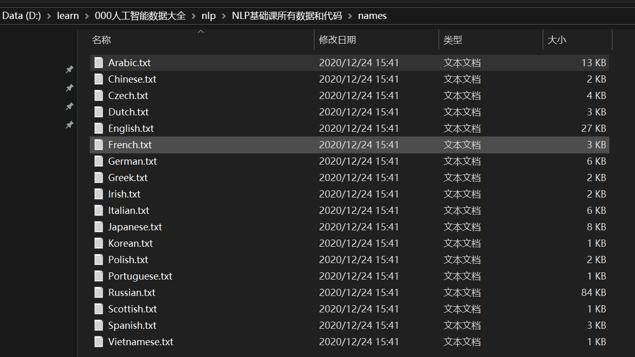
Chinese.txt部分数据预览：

Ang
Au-Yong
Bai
Ban
Bao
Bei
Bian
Bui
Cai
Cao
Cen
Chai
Chaim
Chan
Chang
Chao
Che
Chen
Cheng
Cheung
Chew
Chieu
Chin
Chong

1. 数据预处理与模型构建

1.1 导入必备工具包

import torch
import torch.nn as nn
import torch.optim as optim
import os
import glob
import unicodedata
import random
import time
import matplotlib.pyplot as plt
import matplotlib.ticker as ticker

# 设置随机种子保证可重复性
torch.manual_seed(1)
random.seed(1)

# 检查GPU是否可用
device = torch.device("cuda" if torch.cuda.is_available() else "cpu")
print(f"Using device: {device}")

1.2 数据预处理

# 定义所有可能的字母
all_letters = "abcdefghijklmnopqrstuvwxyzABCDEFGHIJKLMNOPQRSTUVWXYZ .,;'"
n_letters = len(all_letters)


# 字符规范化：将Unicode转换为ASCII
def unicodeToAscii(s):
    """
    将Unicode字符串转换为ASCII字符串
    参数:
        s: 输入的Unicode字符串
    返回:
        规范化后的ASCII字符串
    """
    return ''.join(
        c for c in unicodedata.normalize('NFD', s)
        if unicodedata.category(c) != 'Mn' and c in all_letters
    )


# 测试unicodeToAscii函数
s = "Ślusarski"
print(f"Before normalization: {s}")
print(f"After normalization: {unicodeToAscii(s)}")


# 从文件中读取数据
def readLines(filename):
    """
    从文件中读取每一行并加载到内存中形成列表
    参数:filename: 文件名
    返回:规范化后的人名列表
    """
    lines = open(filename, encoding='utf-8').read().strip().split('\n')#['Abreu', 'Albuquerque', 'Almeida', 'Alves', 'Araújo', 'Araullo', 'Barros', 'Basurto', 'Belo', 'Cabral']
    return [unicodeToAscii(line) for line in lines]#['Abreu', 'Albuquerque', 'Almeida', 'Alves', 'Araujo', 'Araullo', 'Barros', 'Basurto', 'Belo', 'Cabral']


# 加载所有数据
data_path = "D:/learn/000人工智能数据大全/nlp/NLP基础课所有数据和代码/names/"
category_lines = {}  # 字典: {language: [names...]}
all_categories = []  # 所有语言类别列表

# 遍历data_path下的所有txt文件
for filename in glob.glob(data_path + '*.txt'):
    # 获取类别名(去掉.txt后缀)
    category = os.path.splitext(os.path.basename(filename))[0]#Chinese
    all_categories.append(category)
    print("语言类别：",category)
    # 读取文件内容并规范化
    lines = readLines(filename)
    category_lines[category] = lines
n_categories = len(all_categories)
print(f"Total categories: {n_categories}")
print(f"Sample Chinese names: {category_lines['Chinese'][:5]}")

Total categories: 18
Sample Chinese names: ['Ang', 'AuYong', 'Bai', 'Ban', 'Bao']

为什么要将将Unicode转换为ASCII

统一字符表示：Unicode中同一个字符可能有多种表示方式（如'é'可以是一个字符或'e'+重音组合）

分解字符：NFD形式将字符分解为基础字符和组合标记（如'é' → 'e' + '´'）

去除变音符号（Diacritics）
if unicodedata.category(c) != 'Mn' # 过滤掉组合标记
Mn类别：代表"Mark, nonspacing"（非占位组合标记）

保留基础字母：如将'ç'变为'c'，'ü'变为'u'

3. 字符集控制
c in all_letters  # 确保字符在指定范围内
限制字符集：只保留ASCII字母、空格和基本标点（.,;'）

兼容性：确保所有系统都能正确处理，避免特殊字符问题

4. 为什么这对人名分类很重要？

数据一致性：不同语言的人名可能有相同基础字母但不同变音符号（如"Müller"和"Muller"）

简化模型输入：减少字符表大小（从数万Unicode字符→几十个ASCII字符）

提高鲁棒性：避免因编码问题导致的处理错误

实际示例

输入："Ślusàrski"
处理过程：

NFD分解：'Ś' + '′'+'l' + 'u' + 's' + 'à' + '`' +'r' + 's' + 'k' + 'i'

过滤组合标记：移除'Ś'中的重音部分，保留'S'

最终输出："Slusarski"

注意事项

这种转换会丢失部分语言特征（如德语中的变音符号包含语义信息），但在人名分类任务中：

利大于弊（提高泛化能力）

可通过其他特征（如字母组合模式）弥补信息损失

这种预处理是NLP中处理多语言文本的常见做法，特别是在需要简化输入特征的场景中。

1.3 数据转换为张量

def lineToTensor(name_str):
    """
    将人名转换为one-hot张量表示
    参数:line: 输入的人名字符串
    返回:形状为(len(line), 1, n_letters)的张量#n_letters就是：len("abcdefghijklmnopqrstuvwxyzABCDEFGHIJKLMNOPQRSTUVWXYZ .,;'")
    """
    tensor = torch.zeros(len(name_str), 1, n_letters)
    for li, letter in enumerate(name_str):
        tensor[li][0][all_letters.find(letter)] = 1
    return tensor

# 测试lineToTensor函数
name_str = "Bai"
name_str_tensor = lineToTensor(name_str)
print(f"name_str tensor for '{name_str}':")
print(name_str_tensor)
print(f"Shape: {name_str_tensor.shape}")

查看打印结果

name_str tensor for 'Bai':
tensor([[[0., 0., 0., 0., 0., 0., 0., 0., 0., 0., 0., 0., 0., 0., 0., 0., 0.,
          0., 0., 0., 0., 0., 0., 0., 0., 0., 0., 1., 0., 0., 0., 0., 0., 0.,
          0., 0., 0., 0., 0., 0., 0., 0., 0., 0., 0., 0., 0., 0., 0., 0., 0.,
          0., 0., 0., 0., 0., 0.]],

        [[1., 0., 0., 0., 0., 0., 0., 0., 0., 0., 0., 0., 0., 0., 0., 0., 0.,
          0., 0., 0., 0., 0., 0., 0., 0., 0., 0., 0., 0., 0., 0., 0., 0., 0.,
          0., 0., 0., 0., 0., 0., 0., 0., 0., 0., 0., 0., 0., 0., 0., 0., 0.,
          0., 0., 0., 0., 0., 0.]],

        [[0., 0., 0., 0., 0., 0., 0., 0., 1., 0., 0., 0., 0., 0., 0., 0., 0.,
          0., 0., 0., 0., 0., 0., 0., 0., 0., 0., 0., 0., 0., 0., 0., 0., 0.,
          0., 0., 0., 0., 0., 0., 0., 0., 0., 0., 0., 0., 0., 0., 0., 0., 0.,
          0., 0., 0., 0., 0., 0.]]])
Shape: torch.Size([3, 1, 57])

1.4 构建RNN模型

传统RNN模型

class RNN(nn.Module):
    """
    传统RNN模型
    """

    def __init__(self, input_size, hidden_size, output_size, num_layers=1):
        """
        初始化RNN模型
        参数:
            input_size: 输入特征维度
            hidden_size: 隐藏层维度
            output_size: 输出维度
            num_layers: RNN层数
        """
        super(RNN, self).__init__()
        self.hidden_size = hidden_size
        self.num_layers = num_layers

        # 定义RNN层
        self.rnn = nn.RNN(input_size, hidden_size, num_layers)

        # 定义全连接层
        self.fc = nn.Linear(hidden_size, output_size)

        # 定义softmax层
        self.softmax = nn.LogSoftmax(dim=-1)

    def forward(self, input, hidden):
        """
        前向传播
        参数:
            input: 输入张量
            hidden: 隐藏状态
        返回:输出和新的隐藏状态
        """
        # 由于RNN输入必须是3维张量，这里增加一个batch维度 (1, n_letters) -> (1, 1, n_letters)
        input = input.unsqueeze(0)

        # 通过RNN层
        output, hidden = self.rnn(input, hidden)

        # 通过全连接层和softmax
        output = self.fc(output)
        output = self.softmax(output)

        return output, hidden

    def initHidden(self):
        """
        初始化隐藏状态
        返回:
            初始化的隐藏状态张量
        """
        return torch.zeros(self.num_layers, 1, self.hidden_size).to(device)

LSTM模型


class LSTM(nn.Module):
    """
    LSTM模型
    """

    def __init__(self, input_size, hidden_size, output_size, num_layers=1):
        """
        初始化LSTM模型
        参数:
            input_size: 输入特征维度
            hidden_size: 隐藏层维度
            output_size: 输出维度
            num_layers: LSTM层数
        """
        super(LSTM, self).__init__()
        self.hidden_size = hidden_size
        self.num_layers = num_layers

        # 定义LSTM层
        self.lstm = nn.LSTM(input_size, hidden_size, num_layers)

        # 定义全连接层
        self.fc = nn.Linear(hidden_size, output_size)

        # 定义softmax层
        self.softmax = nn.LogSoftmax(dim=-1)

    def forward(self, input, hidden, cell):
        """
        前向传播
        参数:
            input: 输入张量
            hidden: 隐藏状态
            cell: 细胞状态
        返回:
            输出、新的隐藏状态和细胞状态
        """
        input = input.unsqueeze(0)
        output, (hidden, cell) = self.lstm(input, (hidden, cell))
        output = self.fc(output)
        output = self.softmax(output)
        return output, hidden, cell

    def initHiddenAndCell(self):
        """
        初始化隐藏状态和细胞状态
        返回:
            初始化的隐藏状态和细胞状态张量
        """
        hidden = torch.zeros(self.num_layers, 1, self.hidden_size).to(device)
        cell = torch.zeros(self.num_layers, 1, self.hidden_size).to(device)
        return hidden, cell

GRU模型

class GRU(nn.Module):
    """
    GRU模型
    """

    def __init__(self, input_size, hidden_size, output_size, num_layers=1):
        """
        初始化GRU模型
        参数:
            input_size: 输入特征维度
            hidden_size: 隐藏层维度
            output_size: 输出维度
            num_layers: GRU层数
        """
        super(GRU, self).__init__()
        self.hidden_size = hidden_size
        self.num_layers = num_layers

        # 定义GRU层
        self.gru = nn.GRU(input_size, hidden_size, num_layers)

        # 定义全连接层
        self.fc = nn.Linear(hidden_size, output_size)

        # 定义softmax层
        self.softmax = nn.LogSoftmax(dim=-1)

    def forward(self, input, hidden):
        """
        前向传播
        参数:
            input: 输入张量
            hidden: 隐藏状态
        返回:
            输出和新的隐藏状态
        """
        input = input.unsqueeze(0)
        output, hidden = self.gru(input, hidden)
        output = self.fc(output)
        output = self.softmax(output)
        return output, hidden

    def initHidden(self):
        """
        初始化隐藏状态
        返回:
            初始化的隐藏状态张量
        """
        return torch.zeros(self.num_layers, 1, self.hidden_size).to(device)

实例化及调用测试

# 初始化模型参数
input_size = n_letters#all_letters = "abcdefghijklmnopqrstuvwxyzABCDEFGHIJKLMNOPQRSTUVWXYZ .,;'"的长度
hidden_size = 128
output_size = n_categories#要预测的类别总数

# 实例化模型
rnn = RNN(input_size, hidden_size, output_size).to(device)
lstm = LSTM(input_size, hidden_size, output_size).to(device)
gru = GRU(input_size, hidden_size, output_size).to(device)

# 测试模型
input_tensor = lineToTensor('B').squeeze(0).to(device)

# RNN测试
hidden = rnn.initHidden()
rnn_output, next_hidden = rnn(input_tensor, hidden)
print(f"RNN output : {rnn_output}")
print(f"RNN output shape: {rnn_output.shape}")

# LSTM测试
hidden, cell = lstm.initHiddenAndCell()
lstm_output, next_hidden, next_cell = lstm(input_tensor, hidden, cell)
print(f"LSTM output shape: {lstm_output.shape}")

# GRU测试
hidden = gru.initHidden()
gru_output, next_hidden = gru(input_tensor, hidden)
print(f"GRU output shape: {gru_output.shape}")

RNN output : tensor([[[-2.7759, -2.9142, -2.9317, -2.9188, -2.7782, -2.8736, -3.0112, -2.8305, -2.8372, -2.8908, -2.8927, -2.8922, -2.9920, -3.0065, -2.8235, -2.9366, -2.9332, -2.8308]]], grad_fn=<LogSoftmaxBackward0>)
RNN output shape: torch.Size([1, 1, 18])
LSTM output shape: torch.Size([1, 1, 18])
GRU output shape: torch.Size([1, 1, 18])

2. 构建训练函数

2.1 辅助函数

def categoryFromOutput(output):
    """
    从模型输出中获取类别
    参数:
        output: 模型输出张量
    返回:
        类别名称和类别索引
    """
    top_n, top_i = output.topk(1)
    category_i = top_i[0].item()
    return all_categories[category_i], category_i

def randomChoice(l):
    """
    从列表中随机选择一个元素
    参数:
        l: 列表
    返回:
        随机选择的元素
    """
    return l[random.randint(0, len(l) - 1)]

def randomTrainingExample():
    """
    随机选择一个训练样本
    返回:
        类别名称、人名张量、类别索引
    """
    category = randomChoice(all_categories)
    name_str = randomChoice(category_lines[category])
    category_tensor = torch.tensor([all_categories.index(category)], dtype=torch.long).to(device)
    name_str_tensor = lineToTensor(name_str).to(device)
    return category, name_str, category_tensor, name_str_tensor

# 测试随机样本选择
for i in range(3):
    category, name_str, category_tensor, name_str_tensor = randomTrainingExample()
    print(f"Category: {category}, Line: {name_str}")
    print(f"category_tensor: {category_tensor}, name_str_tensor: {name_str_tensor}")

2.2 训练函数

def train(model, criterion, optimizer, category_tensor, name_str_tensor):
    """
    训练模型的一个样本
    参数:
        model: 模型(RNN/LSTM/GRU)
        criterion: 损失函数
        optimizer: 优化器
        category_tensor: 类别张量
        name_str_tensor: 人名张量
    返回:
        输出和损失
    """
    # 初始化隐藏状态
    if isinstance(model, LSTM):
        hidden, cell = model.initHiddenAndCell()
    else:
        hidden = model.initHidden()

    # 将模型梯度归零
    model.zero_grad()

    # 遍历人名的每个字符
    for i in range(name_str_tensor.size()[0]):
        if isinstance(model, LSTM):
            output, hidden, cell = model(name_str_tensor[i], hidden, cell)
        else:
            output, hidden = model(name_str_tensor[i], hidden)

    # 计算损失
    loss = criterion(output.squeeze(0), category_tensor)

    # 反向传播
    loss.backward()

    # 更新参数
    optimizer.step()

    return output, loss.item()


def timeSince(since):
    """
    计算从某个时间点到现在的时间差
    参数:
        since: 起始时间
    返回:
        格式化的时间字符串
    """
    now = time.time()
    s = now - since
    m = int(s / 60)
    s -= m * 60
    return f"{m}m {int(s)}s"


def trainModel(model, model_name, n_iters=100000, print_every=5000, plot_every=1000, learning_rate=0.005):
    """
    训练模型
    参数:
        model: 要训练的模型
        model_name: 模型名称
        n_iters: 训练迭代次数
        print_every: 每隔多少次打印一次信息
        plot_every: 每隔多少次记录一次损失用于绘图
        learning_rate: 学习率
    返回:
        训练过程中的损失列表
    """
    start = time.time()
    current_loss = 0
    all_losses = []

    # 定义损失函数和优化器
    criterion = nn.NLLLoss()
    optimizer = optim.SGD(model.parameters(), lr=learning_rate)

    for iter in range(1, n_iters + 1):
        # 获取随机训练样本
        category, name_str, category_tensor, name_str_tensor = randomTrainingExample()

        # 训练模型
        output, loss = train(model, criterion, optimizer, category_tensor, name_str_tensor)
        current_loss += loss

        # 打印训练信息
        if iter % print_every == 0:
            guess, guess_i = categoryFromOutput(output)
            correct = '✓' if guess == category else f'✗ ({category})'
            print(f"{iter} {iter / n_iters * 100:.1f}% {timeSince(start)} {loss:.4f} {name_str} / {guess} {correct}")

        # 记录损失用于绘图
        if iter % plot_every == 0:
            all_losses.append(current_loss / plot_every)
            current_loss = 0

    # 绘制损失曲线
    plt.figure()
    plt.plot(all_losses)
    plt.title(f'{model_name} Training Loss')
    plt.xlabel('Iterations (x1000)')
    plt.ylabel('Loss')
    plt.show()

    return all_losses


# 训练RNN模型
print("Training RNN...")
rnn_losses = trainModel(rnn, "RNN")

# 训练LSTM模型
print("\nTraining LSTM...")
lstm_losses = trainModel(lstm, "LSTM")

# 训练GRU模型
print("\nTraining GRU...")
gru_losses = trainModel(gru, "GRU")

# 比较三种模型的训练损失
plt.figure(figsize=(10, 6))
plt.plot(rnn_losses, label='RNN')
plt.plot(lstm_losses, label='LSTM')
plt.plot(gru_losses, label='GRU')
plt.title('Comparison of Training Losses')
plt.xlabel('Iterations (x1000)')
plt.ylabel('Loss')
plt.legend()
plt.show()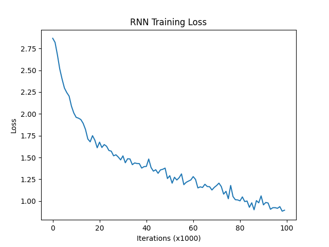

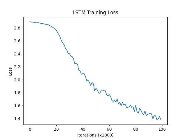
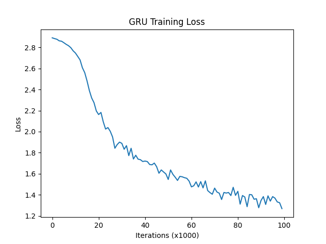
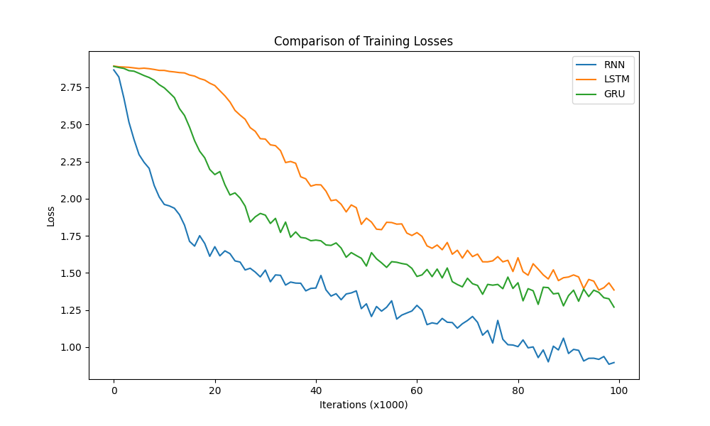
损失对比曲线分析:
模型训练的损失降低快慢代表模型收敛程度,由图可知,传统RNN的模型收敛情况最好,然后是GRU,最后是LSTM,这是因为: 我们当前处理的文本数据是人名,他们的长度有限且长距离字母间基本无特定关联,因此无法发挥改进模型LSTM和GRU的长距离捕捉语义关联的优势。所以在以后的模型选用时,要通过对任务的分析以及实验对比,选择最适合的模型。

点击查看完整训练日志

Training RNN...
5000 5.0% 0m 14s 2.6088 Severins / Greek ✗ (Dutch)
10000 10.0% 0m 28s 0.9120 Phung / Vietnamese ✓
15000 15.0% 0m 42s 0.2584 Matsoukis / Greek ✓
20000 20.0% 0m 57s 2.1118 Sugase / Arabic ✗ (Japanese)
25000 25.0% 1m 11s 0.4751 Henderson / Scottish ✓
30000 30.0% 1m 26s 0.2416 Jong / Korean ✓
35000 35.0% 1m 40s 2.0303 Letsos / Scottish ✗ (Greek)
40000 40.0% 1m 54s 0.7113 Opova / Czech ✓
45000 45.0% 2m 9s 3.3019 Haynes / Arabic ✗ (English)
50000 50.0% 2m 23s 3.0582 Colon / Irish ✗ (Spanish)
55000 55.0% 2m 37s 0.0201 Zouvelekis / Greek ✓
60000 60.0% 2m 52s 2.0891 Bell / Irish ✗ (Scottish)
65000 65.0% 3m 6s 0.8991 Kober / Czech ✓
70000 70.0% 3m 21s 1.0251 Eoin / Irish ✓
75000 75.0% 3m 35s 3.2046 Macdonald / English ✗ (Scottish)
80000 80.0% 3m 49s 0.1424 Karahalios / Greek ✓
85000 85.0% 4m 4s 3.1600 Peers / Portuguese ✗ (English)
90000 90.0% 4m 18s 1.7004 Felix / Spanish ✓
95000 95.0% 4m 33s 0.0310 Dubanowski / Polish ✓
100000 100.0% 4m 47s 0.3119 Piatek / Polish ✓

Training LSTM...
5000 5.0% 0m 24s 2.8998 Auttenberg / Greek ✗ (Polish)
10000 10.0% 0m 48s 2.9027 Bonfils / Japanese ✗ (French)
15000 15.0% 1m 12s 2.8958 Salcedo / Japanese ✗ (Spanish)
20000 20.0% 1m 36s 2.8935 Raske / Czech ✗ (Dutch)
25000 25.0% 2m 0s 2.7027 Machado / Scottish ✗ (Portuguese)
30000 30.0% 2m 24s 2.8205 Santos / Arabic ✗ (Spanish)
35000 35.0% 2m 48s 1.3920 Poplawski / Polish ✓
40000 40.0% 3m 11s 2.2951 Geiger / French ✗ (German)
45000 45.0% 3m 36s 2.8979 Asker / German ✗ (Arabic)
50000 50.0% 3m 59s 2.2894 Kennedy / Dutch ✗ (Scottish)
55000 55.0% 4m 23s 0.4661 Sorrentino / Italian ✓
60000 60.0% 4m 47s 0.3506 Sorrentino / Italian ✓
65000 65.0% 5m 10s 1.1480 Rahal / Arabic ✓
70000 70.0% 5m 34s 1.0543 Shimizu / Japanese ✓
75000 75.0% 5m 57s 0.3870 Tommii / Japanese ✓
80000 80.0% 6m 20s 1.3761 Sanda / Japanese ✓
85000 85.0% 6m 44s 2.3956 Bartosz / Spanish ✗ (Polish)
90000 90.0% 7m 7s 1.5289 Tso / Korean ✗ (Chinese)
95000 95.0% 7m 31s 3.3459 Forbes / Portuguese ✗ (English)
100000 100.0% 7m 54s 1.2309 Rome / French ✓

Training GRU...
5000 5.0% 0m 20s 2.8352 Amatore / Russian ✗ (Italian)
10000 10.0% 0m 41s 2.7114 Can / Irish ✗ (Dutch)
15000 15.0% 1m 1s 2.8145 Machado / Spanish ✗ (Portuguese)
20000 20.0% 1m 22s 2.1758 Freitas / Greek ✗ (Portuguese)
25000 25.0% 1m 42s 0.3820 Sotiris / Greek ✓
30000 30.0% 2m 3s 1.1031 Cui / Chinese ✓
35000 35.0% 2m 24s 1.0792 You / Vietnamese ✗ (Korean)
40000 40.0% 2m 44s 1.1914 Xun / Korean ✗ (Chinese)
45000 45.0% 3m 5s 0.7041 Seok / Korean ✓
50000 50.0% 3m 27s 1.5210 Cunningham / Scottish ✓
55000 55.0% 3m 52s 2.0188 Readman / Scottish ✗ (English)
60000 60.0% 4m 15s 0.9751 Mcdonald / Scottish ✓
65000 65.0% 4m 36s 0.1497 Renov / Russian ✓
70000 70.0% 4m 58s 0.7613 Hama / Japanese ✓
75000 75.0% 5m 20s 0.5726 Kogara / Japanese ✓
80000 80.0% 5m 45s 2.4267 Andres / Portuguese ✗ (German)
85000 85.0% 6m 7s 1.6796 Kerridge / English ✓
90000 90.0% 6m 29s 2.1302 Schoorel / Spanish ✗ (Dutch)
95000 95.0% 6m 51s 0.5340 Sinclair / Scottish ✓
100000 100.0% 7m 13s 0.2052 Okuda / Japanese ✓

训练耗时对比图分析:
模型训练的耗时长短代表模型的计算复杂度,由图可知,也正如我们之前的理论分析,传统RNN复杂度最低,耗时几乎只是后两者的一半,然后是GRU,最后是复杂度最高的LSTM。
结论:
模型选用一般应通过实验对比,并非越复杂或越先进的模型表现越好,而是需要结合自己的特定任务,从对数据的分析和实验结果中获得最佳答案

3. 构建预测函数

def evaluate(model, name_str_tensor):
    """
    评估模型在给定输入上的表现
    参数:
        model: 要评估的模型
        name_str_tensor: 输入人名张量
    返回:
        模型输出
    """
    # 初始化隐藏状态
    if isinstance(model, LSTM):
        hidden, cell = model.initHiddenAndCell()
    else:
        hidden = model.initHidden()

    # 遍历人名的每个字符
    for i in range(name_str_tensor.size()[0]):
        if isinstance(model, LSTM):
            output, hidden, cell = model(name_str_tensor[i], hidden, cell)
        else:
            output, hidden = model(name_str_tensor[i], hidden)

    return output


def predict(model, input_name_str, n_predictions=3):
    """
    使用模型进行预测
    参数:
        model: 要使用的模型
        input_name_str: 输入人名
        n_predictions: 要返回的top N预测结果
    返回:
        预测结果列表
    """
    print(f"\n> {input_name_str}")
    with torch.no_grad():
        output = evaluate(model, lineToTensor(input_name_str).to(device))

        # 调试输出形状和内容
        print(f"Output shape: {output.shape}")  # 应该输出[1,1,18]
        print(f"Output values: {output.squeeze()}")  # 查看实际输出值

        # 修正维度问题：先压缩不必要的维度
        output = output.squeeze()  # 从[1,1,18]变为[18]

        # 确保请求的预测数量不超过类别数
        n_predictions = min(n_predictions, len(all_categories))

        # 获取top N预测结果（在dim=0上操作）
        topv, topi = output.topk(n_predictions, 0, True)

        predictions = []

        for i in range(n_predictions):
            value = topv[i].item()
            category_index = topi[i].item()
            print(f"( {value:.2f}) {all_categories[category_index]}")
            predictions.append([value, all_categories[category_index]])

    return predictions


# 测试预测函数
# 美国名字
predict(rnn, "Jackson")
predict(lstm, "Jackson")
predict(gru, "Jackson")
# 日本名字
predict(rnn, "Satoshi")
predict(lstm, "Satoshi")
predict(gru, "Satoshi")

# 中国名字
predict(rnn, "Zhang")
predict(lstm, "Zhang")
predict(gru, "Zhang")

predict(rnn, "Susan")
predict(lstm, "Susan")
predict(gru, "Susan")

predict(rnn, "luzhanshi")
predict(lstm, "luzhanshi")
predict(gru, "luzhanshi")

# 法国名字
predict(rnn, "Charles André Joseph Marie de Gaulle")
predict(lstm, "Charles André Joseph Marie de Gaulle")
predict(gru, "Charles André Joseph Marie de Gaulle")

点击查看预测结果

> Jackson
Output shape: torch.Size([1, 1, 18])
Output values: tensor([ -7.7283, -15.1358,  -3.6243,  -5.2210,  -1.0218,  -5.3576,  -4.8556,-5.4470,  -6.1742, -10.7871, -11.6995,  -9.4342,  -8.2013, -10.8508,-3.1518,  -0.6061, -10.1330, -17.9064])
( -0.61) Scottish
( -1.02) English
( -3.15) Russian

> Jackson
Output shape: torch.Size([1, 1, 18])
Output values: tensor([ -4.5512, -10.1603,  -3.8185,  -3.4728,  -1.7608,  -5.8610,  -4.2233,-5.0331,  -6.1429,  -8.6363,  -8.3485,  -7.0347,  -4.0323, -10.2805,-3.7613,  -0.3628,  -8.1325, -11.8930])
( -0.36) Scottish
( -1.76) English
( -3.47) Dutch

> Jackson
Output shape: torch.Size([1, 1, 18])
Output values: tensor([ -7.5238,  -8.8740,  -3.3532,  -3.6266,  -2.3916,  -5.8037,  -3.5697,-5.4640,  -7.1469,  -7.0312,  -8.2252,  -4.5493,  -3.2389, -10.3819,-2.5910,  -0.3807,  -7.1692, -13.5724])
( -0.38) Scottish
( -2.39) English
( -2.59) Russian

> Satoshi
Output shape: torch.Size([1, 1, 18])
Output values: tensor([ -5.7750,  -8.9770,  -2.8510,  -6.6472,  -5.8354,  -5.7756,  -5.8914,-8.0980,  -8.7269,  -1.6443,  -0.3406, -12.9274,  -4.4524,  -7.2577,-4.5985, -11.3986,  -6.5155, -10.4883])
( -0.34) Japanese
( -1.64) Italian
( -2.85) Czech

> Satoshi
Output shape: torch.Size([1, 1, 18])
Output values: tensor([ -0.8073, -11.1554,  -6.2725,  -8.4323,  -7.6616,  -6.6945,  -7.0927,-5.4146,  -7.8847,  -2.9668,  -0.7366, -12.7616,  -4.7119,  -6.8010,-5.9150,  -8.4510,  -6.7675,  -9.5558])
( -0.74) Japanese
( -0.81) Arabic
( -2.97) Italian

> Satoshi
Output shape: torch.Size([1, 1, 18])
Output values: tensor([ -1.6525, -10.4843,  -5.3554,  -7.4678,  -8.2391,  -7.1830,  -6.8495,-4.4652,  -7.8201,  -2.9233,  -0.3430, -11.7282,  -4.1148,  -8.4619,-4.8113,  -8.7762,  -7.1180,  -9.7332])
( -0.34) Japanese
( -1.65) Arabic
( -2.92) Italian

> Zhang
Output shape: torch.Size([1, 1, 18])
Output values: tensor([ -9.9794,  -0.3431,  -7.9756,  -8.3555,  -6.7249, -10.5248,  -5.9702,
        -17.0994, -10.8128, -11.6337,  -8.3102,  -1.3966,  -8.6262, -16.5598,-6.8832,  -7.2242, -11.1728,  -3.3135])
( -0.34) Chinese
( -1.40) Korean
( -3.31) Vietnamese

> Zhang
Output shape: torch.Size([1, 1, 18])
Output values: tensor([ -4.6206,  -0.7780,  -5.7530,  -4.7867,  -5.2023,  -6.9409,  -4.3260,
        -10.9132,  -4.4263,  -8.0071,  -5.1054,  -2.0108,  -6.2309, -10.5884,-5.8845,  -4.6250,  -8.5494,  -1.1008])
( -0.78) Chinese
( -1.10) Vietnamese
( -2.01) Korean

> Zhang
Output shape: torch.Size([1, 1, 18])
Output values: tensor([ -5.4885,  -1.0406,  -6.1086,  -4.6721,  -4.0795,  -6.8981,  -3.3706,
        -11.9990,  -3.7337,  -8.7791,  -5.1086,  -2.0592,  -6.0811, -11.4077,-5.8623,  -3.4625,  -9.3958,  -0.9558])
( -0.96) Vietnamese
( -1.04) Chinese
( -2.06) Korean

> Susan
Output shape: torch.Size([1, 1, 18])
Output values: tensor([-6.1677, -4.1831, -3.3016, -3.3740, -2.8176, -5.2211, -3.5468, -7.4435,
        -4.3971, -7.7174, -4.9591, -4.2782, -2.7187, -7.2995, -4.3519, -0.3976,
        -5.1781, -3.6381])
( -0.40) Scottish
( -2.72) Polish
( -2.82) English

> Susan
Output shape: torch.Size([1, 1, 18])
Output values: tensor([-1.1735, -2.0207, -4.0791, -2.3830, -2.8809, -3.1745, -2.5559, -6.6884,
        -3.7211, -6.5325, -5.0317, -3.2705, -4.9640, -6.1109, -5.1304, -2.6679,
        -5.1113, -2.1941])
( -1.17) Arabic
( -2.02) Chinese
( -2.19) Vietnamese

> Susan
Output shape: torch.Size([1, 1, 18])
Output values: tensor([-1.6544, -2.4907, -3.3956, -1.5376, -2.6632, -2.8277, -2.4078, -6.7539,
        -3.5402, -5.1238, -4.2078, -3.8676, -3.8495, -5.3496, -3.9670, -2.2947,
        -4.2242, -3.6378])
( -1.54) Dutch
( -1.65) Arabic
( -2.29) Scottish

> luzhanshi
Output shape: torch.Size([1, 1, 18])
Output values: tensor([ -9.2036,  -8.3343,  -1.8082,  -6.7161,  -3.8666,  -7.6115,  -4.4915,-4.2830,  -7.1130,  -2.5762,  -3.1610,  -9.3789,  -3.1244, -10.7418,-0.4747,  -6.4221,  -6.8615, -13.5123])
( -0.47) Russian
( -1.81) Czech
( -2.58) Italian

> luzhanshi
Output shape: torch.Size([1, 1, 18])
Output values: tensor([-1.6621, -8.8901, -4.0941, -6.6199, -5.3680, -6.7587, -4.7679, -4.2109,
        -5.9299, -2.1025, -0.8158, -9.0834, -3.3109, -7.2002, -1.9092, -5.3442,
        -5.2798, -7.6777])
( -0.82) Japanese
( -1.66) Arabic
( -1.91) Russian

> luzhanshi
Output shape: torch.Size([1, 1, 18])
Output values: tensor([-2.0611, -6.8596, -3.4629, -5.8511, -4.8760, -5.8102, -3.7236, -3.2888,
        -4.2160, -2.0960, -1.3844, -5.5531, -3.7010, -7.9435, -1.0993, -4.4624,
        -5.9794, -6.8356])
( -1.10) Russian
( -1.38) Japanese
( -2.06) Arabic

> Charles André Joseph Marie de Gaulle
Output shape: torch.Size([1, 1, 18])
Output values: tensor([ -9.0547, -13.3042,  -4.7085,  -2.2298,  -1.0208,  -2.4804,  -1.6292,-7.4276,  -1.8712,  -3.2741,  -9.4051,  -9.7947,  -6.7794,  -8.1453,-3.5070,  -4.1638,  -5.5915, -11.0725])
( -1.02) English
( -1.63) German
( -1.87) Irish

> Charles André Joseph Marie de Gaulle
Output shape: torch.Size([1, 1, 18])
Output values: tensor([-10.5133, -12.2635,  -4.1649,  -3.7837,  -3.8238,  -1.4161,  -5.4175,-3.3364,  -0.9791,  -2.2459,  -8.9872, -11.8955,  -8.0392,  -3.6554,-3.0721,  -5.0941,  -2.3354,  -8.5890])
( -0.98) Irish
( -1.42) French
( -2.25) Italian

> Charles André Joseph Marie de Gaulle
Output shape: torch.Size([1, 1, 18])
Output values: tensor([-1.4408e+01, -1.5209e+01, -9.9442e+00, -8.7536e+00, -5.8942e+00,
        -4.9302e+00, -9.8018e+00, -7.4339e+00, -1.4131e-02, -7.2010e+00,
        -1.1776e+01, -1.4152e+01, -1.5019e+01, -9.2337e+00, -7.7469e+00,
        -6.6239e+00, -7.9238e+00, -8.4041e+00])
( -0.01) Irish
( -4.93) French
( -5.89) English

4. 构建评估函数和混淆矩阵

评估函数


def evaluateModel(model, n_examples=10000):
    """
    评估模型在测试集上的表现
    参数:
        model: 要评估的模型
        n_examples: 要评估的样本数量
    返回:
        准确率
    """
    correct = 0

    for _ in range(n_examples):
        category, name_str, category_tensor, name_str_tensor = randomTrainingExample()
        output = evaluate(model, name_str_tensor)
        guess, guess_i = categoryFromOutput(output)
        if guess == category:
            correct += 1

    accuracy = correct / n_examples
    print(f"Model Accuracy: {accuracy * 100:.2f}%")
    return accuracy


# 评估三个模型
print("Evaluating RNN...")
rnn_accuracy = evaluateModel(rnn)

print("\nEvaluating LSTM...")
lstm_accuracy = evaluateModel(lstm)

print("\nEvaluating GRU...")
gru_accuracy = evaluateModel(gru)

Evaluating RNN...
Model Accuracy: 71.64%

Evaluating LSTM...
Model Accuracy: 54.24%

Evaluating GRU...
Model Accuracy: 55.18%

混淆矩阵

# 构建混淆矩阵
def plotConfusionMatrix(model, n_examples=1000):
    """
    绘制混淆矩阵
    参数:
        model: 要评估的模型
        n_examples: 要评估的样本数量
    """
    # 初始化混淆矩阵
    confusion = torch.zeros(n_categories, n_categories)

    for _ in range(n_examples):
        category, name_str, category_tensor, name_str_tensor = randomTrainingExample()
        output = evaluate(model, name_str_tensor)
        guess, guess_i = categoryFromOutput(output)
        category_i = all_categories.index(category)
        confusion[category_i][guess_i] += 1
    '''
    category_i：真实类别的索引（来自randomTrainingExample随机选取的真实标签）
    guess_i：模型预测的类别索引（来自categoryFromOutput）
    只有当两者相等时才会在对角线上累加
    假设评估1000个样本后：
             Predicted
         Eng  Jap  Chi
Actual Eng 900   50   50
       Jap  30  920   50 
       Chi  20   30  950
    '''
    # 归一化混淆矩阵
    # 将每行的值转换为概率，使所有的值范围变为0-1，对角线上的概率值表示分类准确率。
    for i in range(n_categories):
        confusion[i] = confusion[i] / confusion[i].sum()

    # 设置图形
    fig = plt.figure(figsize=(10, 10))
    ax = fig.add_subplot(111)
    cax = ax.matshow(confusion.numpy())
    fig.colorbar(cax)

    # 设置坐标轴
    ax.set_xticks(range(n_categories))
    ax.set_yticks(range(n_categories))
    ax.set_xticklabels(all_categories, rotation=90)
    ax.set_yticklabels(all_categories)

    # 设置标签
    ax.set_xlabel('Predicted')
    ax.set_ylabel('Actual')
    if isinstance(model, LSTM):
         plt.title('LSTM Confusion Matrix')
    elif isinstance(model, GRU):
         plt.title('GRU Confusion Matrix')
    else:
        plt.title('RNN Confusion Matrix')
    plt.show()


# 绘制RNN的混淆矩阵
print("RNN Confusion Matrix:")
plotConfusionMatrix(rnn)

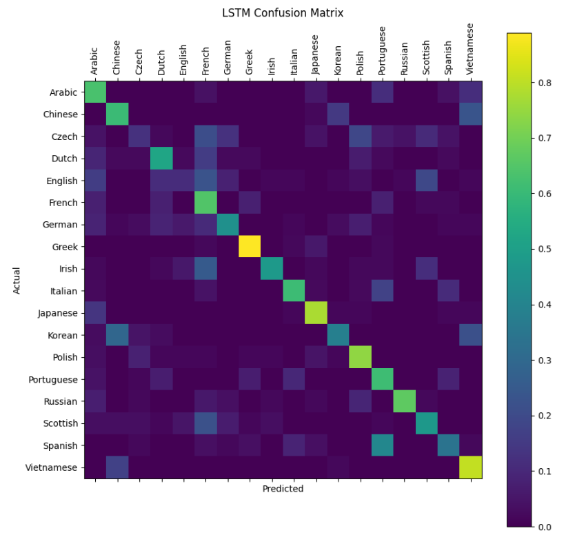
# 绘制LSTM的混淆矩阵
print("LSTM Confusion Matrix:")
plotConfusionMatrix(lstm)

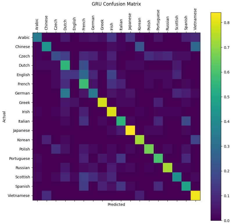
# 绘制GRU的混淆矩阵
print("GRU Confusion Matrix:")
plotConfusionMatrix(gru)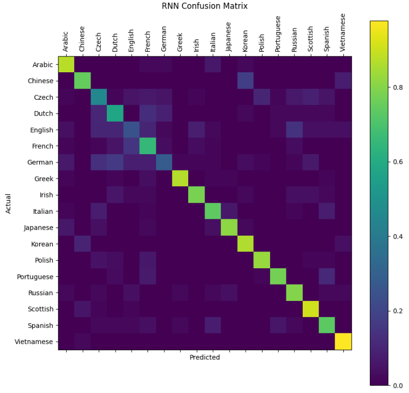

对角线元素 $P (i ∣ i)$ 表示真实类别为 i 时的正确分类概率（召回率/recall）
非对角线元素 $P (j ∣ i)$ 表示将类别 i 误分类为 j 的概率

总结：

混淆矩阵对角线是正确分类
非对角线是各类别间的混淆情况
好的模型会使对角线值明显大于其他位置

这个设计正是为了直观展示模型在哪些类别上容易混淆（比如西班牙语和葡萄牙语名字可能容易互相误判）。

关键概念区分

行归一化（实际类别视角）：

关注模型对每个真实类别的识别能力

对角线表示召回率（Recall）【上面的案例】confusion[i] = confusion[i] / confusion[i].sum()

列归一化（预测类别视角）：

如果对列归一化，对角线表示精确率（Precision）

代码实现：confusion[:,j] = confusion[:,j] / confusion[:,j].sum()

全局归一化：

所有元素除以总样本数

表示联合概率分布
def global_normalize(confusion):
    """
    全局归一化
    整个矩阵除以总样本数
    表示联合概率分布P(真实类别, 预测类别)【真是类别是A的情况下，预测类别是A、B/C...的概率】
    """
    total = confusion.sum()
    return confusion / total if total > 0 else confusion

# 示例输出：
# tensor([[0.2500, 0.0500, 0.0250],  # P(真实=0, 预测=*)
#         [0.1000, 0.3000, 0.0500],  # P(真实=1, 预测=*)
#         [0.0250, 0.0250, 0.1500]]) # P(真实=2, 预测=*)
# 所有元素之和为1.0

5. 保存和加载模型

# 保存模型
def saveModel(model, model_name):
    """
    保存模型到文件
    参数:
        model: 要保存的模型
        model_name: 模型名称
    """
    torch.save(model.state_dict(), f"{model_name}.pth")
    print(f"Model saved to {model_name}.pth")

saveModel(rnn, "rnn_model")
saveModel(lstm, "lstm_model")
saveModel(gru, "gru_model")

# 加载模型
def loadModel(model_class, model_name, input_size, hidden_size, output_size):
    """
    从文件加载模型
    参数:
        model_class: 模型类
        model_name: 模型名称
        input_size: 输入尺寸
        hidden_size: 隐藏层尺寸
        output_size: 输出尺寸
    返回:
        加载的模型
    """
    model = model_class(input_size, hidden_size, output_size).to(device)
    model.load_state_dict(torch.load(f"{model_name}.pth"))
    model.eval()
    print(f"Model loaded from {model_name}.pth")
    return model

# 测试加载模型
loaded_rnn = loadModel(RNN, "rnn_model", input_size, hidden_size, output_size)
predict(loaded_rnn, "Jackson")

总结

本教程完整实现了基于RNN、LSTM和GRU的人名分类器，包括：

数据预处理：读取数据、字符规范化、转换为张量
模型构建：实现了三种循环神经网络模型
训练过程：实现了训练函数和训练循环
评估和预测：实现了模型评估、预测和混淆矩阵可视化
模型保存和加载

通过比较可以发现，LSTM和GRU模型通常比传统RNN表现更好，训练损失下降更快，最终准确率更高。在实际应用中，可以根据需求选择适合的模型。

这个案例展示了如何使用PyTorch构建循环神经网络来解决实际的分类问题，可以扩展到其他类似的序列分类任务中。

posted @ 2025-07-16 15:42 指尖下的世界阅读(17) 评论(0) 收藏举报

刷新页面返回顶部

指尖下的世界

今日事今日毕,今日无事早休息.