11.神经网络案例-mnist手写数字识别
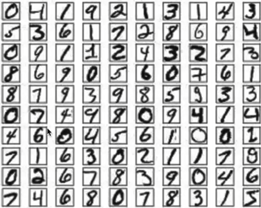
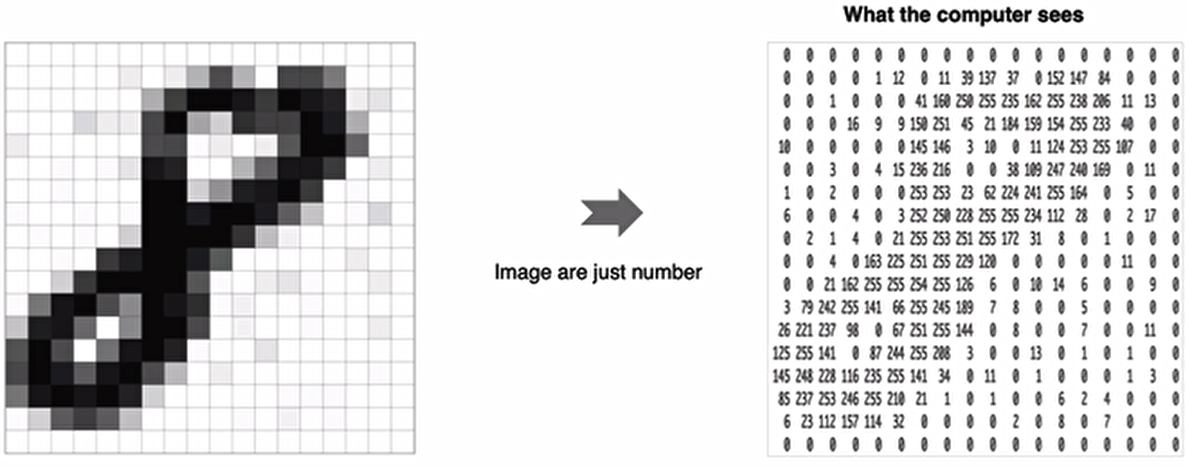
使用手写数字的MNIST数据集如上图所示,该数据集包含60,000个用于训练的样本和10,000个用于测试的样本,图像是固定大小(28x28像素),其值为0到255。
📊 MNIST 数据集基本信息
| 数据集 | 样本数 | 图像大小 | 数据类型 |
|---|---|---|---|
| 训练集 | 60,000 | 28×28 像素 | uint8 (0-255) |
| 测试集 | 10,000 | 28×28 像素 | uint8 (0-255) |
| 标签范围 | 0-9 (手写数字) |
- 数据加载
- 数据处理
- 模型构建
- 模型训练
- 模型测试
- 模型保存
首先要导入所需的工具包:
import numpy as np
import matplotlib.pyplot as plt
plt.rcParams['figure.figsize']=(7,7)
# 数据集
from tensorflow.keras.datasets import mnist
# 构建序列模型
from tensorflow.keras import Sequential
# 导入需要的层
from tensorflow.keras.layers import Dense,Input,Activation,Dropout,BatchNormalization
# 导入辅助工具包
from tensorflow.keras import utils
# 正则化
from tensorflow.keras import regularizers
数据加载与查看
# 数据加载
# 首先加载手写数字图像
nb_class=10
# 加载数据集
# 正确写法:获取两个元组并解包
(x_train, y_train), (x_test, y_test)=mnist.load_data()#注意:mnist.load_data() 函数返回的是一个包含 两个元组 的结构:(x_train, y_train), (x_test, y_test)
x_train.shape,y_train.shape,x_test.shape, y_test.shape#((60000, 28, 28), (60000,), (10000, 28, 28), (10000,))Downloading data from https://storage.googleapis.com/tensorflow/tf-keras-datasets/mnist.npz
4775936/11490434 ━━━━━━━━━━━━━━━━━━━━ 32s 5us/step# 数据展示:将数据集的前9个数据进行展示
for i in range(9):
plt.subplot(3,3,i+1)
plt.imshow(x_train[i])
# 输出对应的目标值
plt.title(y_train[i]) 数据处理
数据处理
神经网络中的每个训练样本是一个向量,因此需要对输入进行重塑,使每个28x28的图像成为一个784维的向量。另外,将输入数据进行归一化处理,从0-255调整到0-1。
可以对比参照:https://www.cnblogs.com/luzhanshi/articles/18924883中的数据集格式
特征值处理:
# 调整数据维度,每一个数字转化为一个向量
x_train=x_train.reshape(60000,784)
x_test=x_test.reshape(10000,784)
# 格式转换
x_train=x_train.astype(np.float32)
x_test=x_test.astype(np.float32)
# 归一化
x_train / = 255
x_test / = 255
# 查看处理后数据
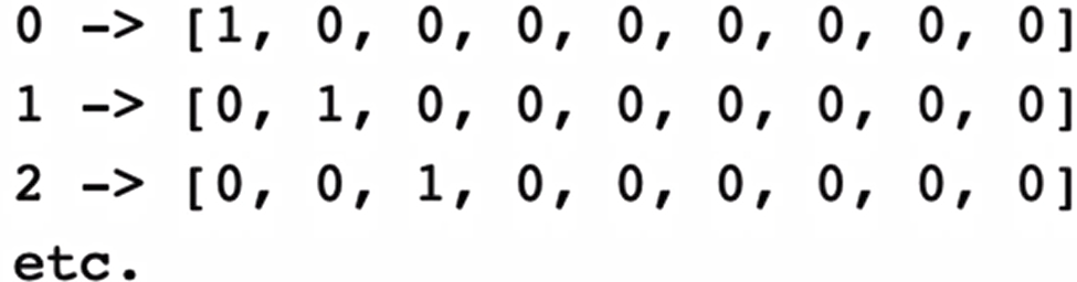
x_train.shape,x_test.shape#((60000, 784), (10000, 784))另外对于目标值我们也需要进行处理,将其转换为热编码的形式:
代码实现:
y_train=utils.to_categorical(y_train,nb_class)
y_test=utils.to_categorical(y_test,nb_class)
y_train.shape,y_test.shape#((60000, 10), (10000, 10))
y_train[0:5]
array([[0., 0., 0., 0., 0., 1., 0., 0., 0., 0.],
[1., 0., 0., 0., 0., 0., 0., 0., 0., 0.],
[0., 0., 0., 0., 1., 0., 0., 0., 0., 0.],
[0., 1., 0., 0., 0., 0., 0., 0., 0., 0.],
[0., 0., 0., 0., 0., 0., 0., 0., 0., 1.]])模型构建
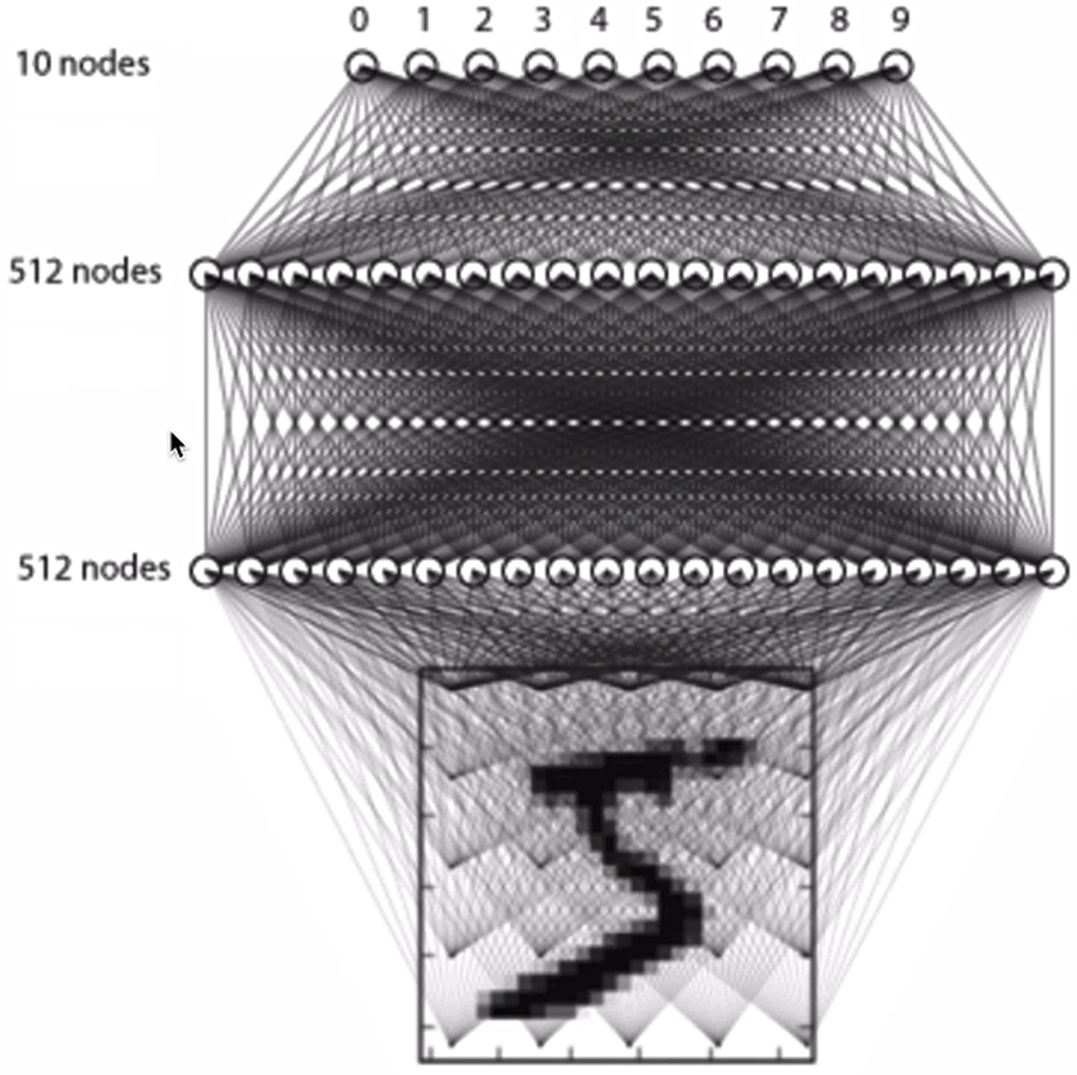
这里我们只构建有3层全连接的网络来进行处理
构建方法如下所示:
#利用模型序列来构建模型
model=Sequential()
# 输入层,输入维度大小为784
model.add(Input(shape=(784,)))
# 全连接层1,共512个神经元,
model.add(Dense(512))
# 添加激活函数
model.add(Activation('relu'))
# 使用正则化方法Dropout,随机失活
model.add(Dropout(0.2))
# 全连接层2,共512个神经元,并加入l2正则化
model.add(Dense(512,kernel_regularizer=regularizers.l2(0.02)))
# BN层
model.add(BatchNormalization())
# 激活函数
model.add(Activation('relu'))
# 使用正则化方法Dropout,随机失活
model.add(Dropout(0.2))
# 输出层,共10个神经元(对应10种分类结果)
model.add(Dense(10))
# softmax将神经网络输出的score转化为概率值
model.add(Activation('softmax'))
model.summary()
Model: "sequential_1"
┏━━━━━━━━━━━━━━━━━━━━━━━━━━━━━━━━━━━━━━┳━━━━━━━━━━━━━━━━━━━━━━━━━━━━━┳━━━━━━━━━━━━━━━━━┓
┃ Layer (type) ┃ Output Shape ┃ Param # ┃
┡━━━━━━━━━━━━━━━━━━━━━━━━━━━━━━━━━━━━━━╇━━━━━━━━━━━━━━━━━━━━━━━━━━━━━╇━━━━━━━━━━━━━━━━━┩
│ dense_1 (Dense) │ (None, 512) │ 401,920 │
├──────────────────────────────────────┼─────────────────────────────┼─────────────────┤
│ activation_1 (Activation) │ (None, 512) │ 0 │
├──────────────────────────────────────┼─────────────────────────────┼─────────────────┤
│ dropout_1 (Dropout) │ (None, 512) │ 0 │
├──────────────────────────────────────┼─────────────────────────────┼─────────────────┤
│ dense_2 (Dense) │ (None, 512) │ 262,656 │
├──────────────────────────────────────┼─────────────────────────────┼─────────────────┤
│ batch_normalization │ (None, 512) │ 2,048 │
│ (BatchNormalization) │ │ │
├──────────────────────────────────────┼─────────────────────────────┼─────────────────┤
│ activation_2 (Activation) │ (None, 512) │ 0 │
├──────────────────────────────────────┼─────────────────────────────┼─────────────────┤
│ dropout_2 (Dropout) │ (None, 512) │ 0 │
├──────────────────────────────────────┼─────────────────────────────┼─────────────────┤
│ dense_3 (Dense) │ (None, 10) │ 5,130 │
├──────────────────────────────────────┼─────────────────────────────┼─────────────────┤
│ activation_3 (Activation) │ (None, 10) │ 0 │
└──────────────────────────────────────┴─────────────────────────────┴─────────────────┘
Total params: 671,754 (2.56 MB)
Trainable params: 670,730 (2.56 MB)
Non-trainable params: 1,024 (4.00 KB)模型编译
设置模型训练使用的损失函数交叉熵损失和优化方法adam,损失函数用来衡量预测值与真实值之间的差异,优化器用来使用损失函数达到最优:
# 模型编译:指定损失函数、优化器、评估方法
model.compile(loss='categorical_crossentropy',optimizer='adam',metrics=['accuracy'])
# 模型编译:等价写法
model.compile(loss=tf.keras.losses.categorical_crossentropy,optimizer=tf.keras.optimizers.Adam(),metrics=tf.keras.metrics.Accuracy())
模型训练
# batch_size:每次送入模型的参数,epochs:所有样本的迭代次数,validation_data:指定验证数据集
history=model.fit(x_train,y_train,batch_size=128,epochs=4,verbose=1,validation_data=(x_test,y_test))
训练过程如下:
Epoch 1/4
469/469 ━━━━━━━━━━━━━━━━━━━━ 4s 6ms/step - accuracy: 0.8736 - loss: 3.1170 - val_accuracy: 0.9580 - val_loss: 0.3342
Epoch 2/4
469/469 ━━━━━━━━━━━━━━━━━━━━ 3s 6ms/step - accuracy: 0.9551 - loss: 0.2863 - val_accuracy: 0.9679 - val_loss: 0.2355
Epoch 3/4
469/469 ━━━━━━━━━━━━━━━━━━━━ 3s 7ms/step - accuracy: 0.9641 - loss: 0.2422 - val_accuracy: 0.9652 - val_loss: 0.2489
Epoch 4/4
469/469 ━━━━━━━━━━━━━━━━━━━━ 3s 6ms/step - accuracy: 0.9683 - loss: 0.2208 - val_accuracy: 0.9723 - val_loss: 0.2199
打印history数据:
history.history{'accuracy': [0.9212333559989929,0.9562000036239624,0.9629833102226257,0.9670666456222534],
'loss': [1.230934739112854,0.2810131907463074,0.24591435492038727,0.22761961817741394],
'val_accuracy': [0.9580000042915344,0.9678999781608582,0.9652000069618225,0.9722999930381775],
'val_loss': [0.33420270681381226,0.23554934561252594,0.24887068569660187,0.21987192332744598]}将损失绘制成曲线:
#绘制损失函数变化曲线
plt.figure()
# 绘制训练集的损失
plt.plot(history.history['loss'],label='train_loss')
#绘制测试集的损失
plt.plot(history.history['val_loss'],label='val_loss')
plt.legend()
plt.grid()
plt.show()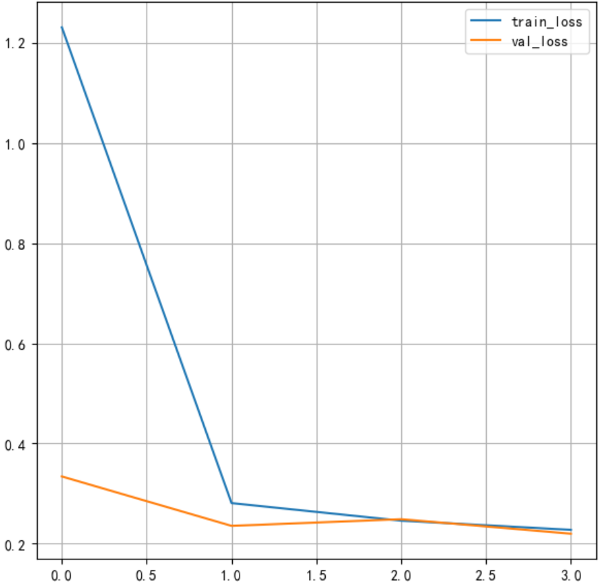
将训练的准确率绘制成曲线:
#绘制准确率变化曲线
plt.figure()
#训练集准确率
plt.plot(history.history['accuracy'],label='train_loss')
#测试集准确率
plt.plot(history.history['val_accuracy'],label='val_loss')
plt.legend()
plt.grid()
plt.show()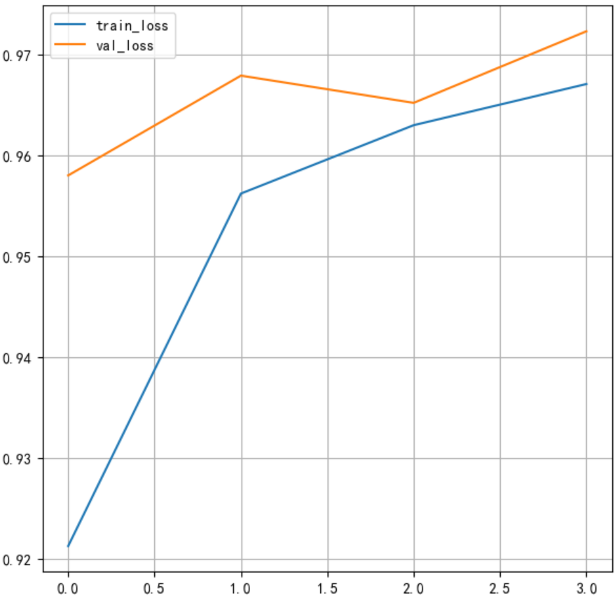
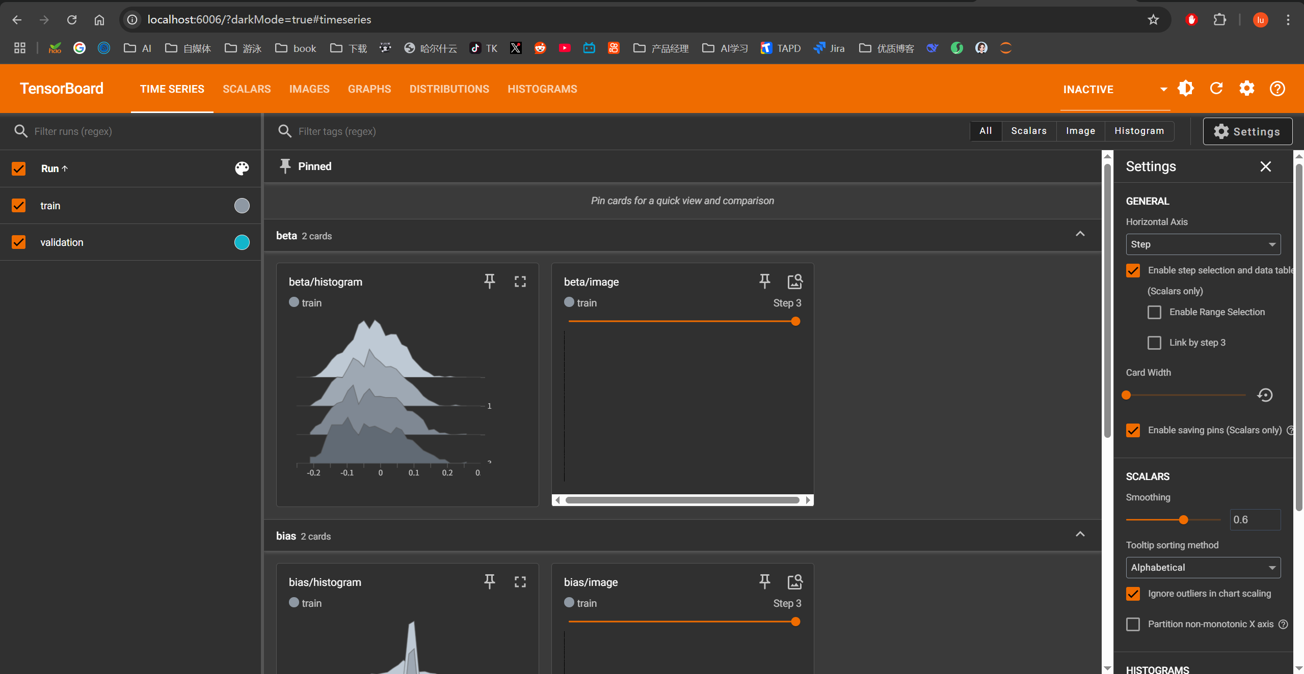
tensorboard监控训练过程
另外可通过tensorboard监控训练过程,这时我们指定回调函数:
# 添加TensorBoard观察
tensorboard=tf.keras.callbacks.TensorBoard(log_dir= r'D:\data\jupyter\Test',histogram_freq=1,write_graph=True,write_images=True)
'''注意:log_dir路径,要求全英文,否则可能会报错'''
再进行训练:
# 模型训练,并指定TensorBoard
history=model.fit(x_train,y_train,batch_size=128,epochs=4,verbose=1,validation_data=(x_test,y_test),callbacks=[tensorboard])打开终端,进入log_dir指定的目录(D:\data\jupyter\Test),执行命令:tensorboard --logdir "D:/data/jupyter/Test/TensorBoard":
D:\data\jupyter\Test\TensorBoard>tensorboard --logdir "D:/data/jupyter/Test/TensorBoard"
2025-06-28 18:56:53.727954: I tensorflow/core/util/port.cc:153] oneDNN custom operations are on. You may see slightly different numerical results due to floating-point round-off errors from different computation orders. To turn them off, set the environment variable `TF_ENABLE_ONEDNN_OPTS=0`.
2025-06-28 18:56:54.648216: I tensorflow/core/util/port.cc:153] oneDNN custom operations are on. You may see slightly different numerical results due to floating-point round-off errors from different computation orders. To turn them off, set the environment variable `TF_ENABLE_ONEDNN_OPTS=0`.
Serving TensorBoard on localhost; to expose to the network, use a proxy or pass --bind_all
TensorBoard 2.18.0 at http://localhost:6006/ (Press CTRL+C to quit)
注意:如果遇到报错,极有可能是TensorBoard 已安装(版本 2.18.0),但系统无法找到可执行文件。这是因为 Python 用户安装目录没有添加到系统 PATH 中。
永久解决方案:添加环境变量
手动添加环境变量:
- Win + R →
sysdm.cpl→ 高级 → 环境变量- 在"系统变量"找到
Path→ 编辑- 新建一项:
C:\Users\luzhanshi\AppData\Roaming\Python\Python312\Scripts- 确定保存所有更改
通过命令提示符添加:
setx PATH "%PATH%;C:\Users\luzhanshi\AppData\Roaming\Python\Python312\Scripts"
在浏览器中打开上面指定的网址,可以查看损失函数和准确率的变化,图结构等。
模型评估
#模型测试
score=model.evaluate(x_test,y_test,verbose=1)
# 打印结果
print(score)
313/313 ━━━━━━━━━━━━━━━━━━━━ 1s 2ms/step - accuracy: 0.9736 - loss: 0.2011
[0.18996557593345642, 0.9754999876022339]模型保存
#保存模型架构与权重到h5文件中
model.save('./mnist_model.h5')
#加载模型,包括架构与权重
model=tf.keras.models.load_model('./mnist_model.h5')
model.summary()
上述代码可以保存成功,但是会有警告:
WARNING:absl:You are saving your model as an HDF5 file via `model.save()` or `keras.saving.save_model(model)`. This file format is considered legacy. We recommend using instead the native Keras format, e.g. `model.save('my_model.keras')` or `keras.saving.save_model(model, 'my_model.keras')`.
WARNING:absl:Compiled the loaded model, but the compiled metrics have yet to be built. `model.compile_metrics` will be empty until you train or evaluate the model.
解决模型保存为HDF5格式时出现警告的问题
这个警告是TensorFlow/Keras在鼓励您使用新的模型保存格式(.keras)替代传统的HDF5格式(.h5)。
原因分析
-
Keras格式(.keras)是新的默认格式
- 这是Keras 3.x的新功能,也被集成到TensorFlow 2.12+版本中
- HDF5格式(.h5)已被标记为"legacy"(传统格式)
-
推荐使用新格式的优势:
- 更简洁的单一文件格式(HDF5实际是复杂的容器格式)
- 更可靠地保存和恢复模型配置
- 更好的向前兼容性
- 支持保存所有自定义对象(层、损失函数等)而不需要
custom_objects参数
解决方案
1. 使用新的Keras格式保存模型(推荐)
# 使用新格式保存
model.save('./mnist_model.keras')
# 加载模型
loaded_model = tf.keras.models.load_model('./mnist_model.keras')
2. 保存为TensorFlow标准格式
tf.saved_model.save(model, r"D:\data\jupyter\Test\model_save")  # ✅ 明确使用 tf.saved_model 模块
# 加载模型
loaded_model = tf.saved_model.load(r'D:\data\jupyter\Test\model_save')
此方法多次尝试,各种报错,做个了解即可
格式对比表
| 格式 | 扩展名 | 特点 | 适用场景 |
|---|---|---|---|
| Keras格式 | .keras | 单一文件,轻量简单,推荐新项目 | 所有新项目 |
| TensorFlow SavedModel | 无特定扩展名(目录) | 包含完整资源,可部署 | TensorFlow Serving, TensorFlow Lite |
| HDF5 (Legacy) | .h5 | 复杂容器格式,向后兼容 | 需要兼容旧代码的场景 |
迁移建议
新项目:始终使用.keras格式
需要部署的场景:使用SavedModel格式
共享模型给使用旧TF版本的用户:同时保存两种格式
# 保存新格式
model.save('latest_model.keras')

# 保存旧格式用于兼容
with keras.suppress_saved_model_warnings():
    model.save('compatible_model.h5')
何时必须使用HDF5格式
虽然不推荐,但在以下场景仍需使用HDF5:
- 需要支持TensorFlow 2.11或更早版本
- 需要与旧版Keras或PyTorch等框架交互
- 需要在某些不支持新格式的库中使用(如某些可视化工具)

 浙公网安备 33010602011771号