kaggle-奥托集团产品分类挑战赛-数据不均衡处理、欠采样、随机森林、模型超参数分析、模型调优

比赛官网链接：https://www.kaggle.com/c/otto-group-product-classification-challenge/overview

背景介绍

奥托集团是世界上最⼤的电⼦商务公司之⼀，在20多个国家设有⼦公司。该公司每天都在世界各地销售数百万种产品,所以对其产品根据性能合理的分类⾮常重要。

不过,在实际⼯作中,⼯作⼈员发现,许多相同的产品得到了不同的分类。本案例要求,你对奥拓集团的产品进⾏正确的分分类。尽可能的提供分类的准确性。

数据简介

本案例中，数据集包含⼤约200,000种产品的93个特征。
所有产品共被分成九个类别（例如时装，电⼦产品等）。

	id	feat_1	feat_4	feat_5	feat_6	feat_7	feat_8	...	feat_85	feat_86	feat_87	feat_90	target
0	1	1	0	0	0	0	0	...	1	0	0	0	Class_1
1	2	0	0	0	0	0	1	...	0	0	0	0	Class_1
2	3	0	0	0	0	0	1	...	0	0	0	0	Class_2
3	4	1	1	6	1	5	0	...	0	1	2	0	Class_1
4	5	0	0	0	0	0	0	...	1	0	0	1	Class_3

竞赛规则

其⽬的是建⽴⼀个能够区分otto公司主要产品类别的预测模型。

获胜的模型将被开源。

评分标准

本案例中，最后结果使⽤多分类对数损失进⾏评估（sklearn有现成的方法）。

具体公式：

上公式中，

其中 N 是测试集中产品的数量，M 是类标签的数量，log 是自然对数。

i表示样本，j表示类别。P_ij代表第i个样本属于类别j的概率。

如果第i个样本真的属于类别j，则y_ij等于1，否则为0。

根据上公式，假如你将所有的测试样本都正确分类，所有p_ij都是1，那每个log(p_ij)都是0，最终的logloss也是0。

假如第1个样本本来是属于1类别的，但是你给它的类别概率p_ij=0.1，那logloss就会累加上log(0.1)这⼀项。我们知道这⼀项是负数，⽽且p_ij越⼩，负得越多，logloss越大，如果p_ij=0，将是⽆穷。这会导致这种情况：你分错了⼀个，logloss就是⽆穷。这当然不合理，为了避免对数函数的极值，我们对⾮常⼩的值做如下处理：

也就是说最⼩不会⼩于10^-15。

实现过程

流程分析

获取数据
- 数据基本处理
- 数据量⽐较⼤，尝试是否可以进⾏数据分割
- 转换⽬标值表示⽅式
模型训练
- 模型基本训练

读取数据

import pandas as pd
# 获取数据
data=pd.read_csv(r"D:\learn\000人工智能数据大全\经典数据集\奥托集团产品分类挑战赛\train.csv")
data.head()

	id	feat_1	feat_4	feat_5	feat_6	feat_7	feat_8	...	feat_85	feat_86	feat_87	feat_90	target
0	1	1	0	0	0	0	0	...	1	0	0	0	Class_1
1	2	0	0	0	0	0	1	...	0	0	0	0	Class_1
2	3	0	0	0	0	0	1	...	0	0	0	0	Class_2
3	4	1	1	6	1	5	0	...	0	1	2	0	Class_1
4	5	0	0	0	0	0	0	...	1	0	0	1	Class_3

查看数据基本情况

data.shape#(61878, 95)
data.describe()

	id	feat_1	feat_2	feat_3	feat_4	feat_5	feat_6	feat_7	feat_8	feat_9	...	feat_84	feat_85	feat_86	feat_87	feat_88	feat_89	feat_90	feat_91	feat_92	feat_93
count	61878.000000	61878.00000	61878.000000	61878.000000	61878.000000	61878.000000	61878.000000	61878.000000	61878.000000	61878.000000	...	61878.000000	61878.000000	61878.000000	61878.000000	61878.000000	61878.000000	61878.000000	61878.000000	61878.000000	61878.000000
mean	30939.500000	0.38668	0.263066	0.901467	0.779081	0.071043	0.025696	0.193704	0.662433	1.011296	...	0.070752	0.532306	1.128576	0.393549	0.874915	0.457772	0.812421	0.264941	0.380119	0.126135
std	17862.784315	1.52533	1.252073	2.934818	2.788005	0.438902	0.215333	1.030102	2.255770	3.474822	...	1.151460	1.900438	2.681554	1.575455	2.115466	1.527385	4.597804	2.045646	0.982385	1.201720
min	1.000000	0.00000	0.000000	0.000000	0.000000	0.000000	0.000000	0.000000	0.000000	0.000000	...	0.000000	0.000000	0.000000	0.000000	0.000000	0.000000	0.000000	0.000000	0.000000	0.000000
25%	15470.250000	0.00000	0.000000	0.000000	0.000000	0.000000	0.000000	0.000000	0.000000	0.000000	...	0.000000	0.000000	0.000000	0.000000	0.000000	0.000000	0.000000	0.000000	0.000000	0.000000
50%	30939.500000	0.00000	0.000000	0.000000	0.000000	0.000000	0.000000	0.000000	0.000000	0.000000	...	0.000000	0.000000	0.000000	0.000000	0.000000	0.000000	0.000000	0.000000	0.000000	0.000000
75%	46408.750000	0.00000	0.000000	0.000000	0.000000	0.000000	0.000000	0.000000	1.000000	0.000000	...	0.000000	0.000000	1.000000	0.000000	1.000000	0.000000	0.000000	0.000000	0.000000	0.000000
max	61878.000000	61.00000	51.000000	64.000000	70.000000	19.000000	10.000000	38.000000	76.000000	43.000000	...	76.000000	55.000000	65.000000	67.000000	30.000000	61.000000	130.000000	52.000000	19.000000	87.000000

8 rows × 94 columns

#查看数据分布是否均匀
import seaborn as sns
import matplotlib.pyplot as plt
sns.countplot(data,x='target',hue='target')
plt.show()

由上图可以看出,该数据类别不均衡,所以需要后期处理

数据基本处理

数据已经经过脱敏,不再需要特殊处理

截取部分数据

尝试简单截取方法

cutdata=data.loc[:9999]
cutdata.shape#(10000, 95)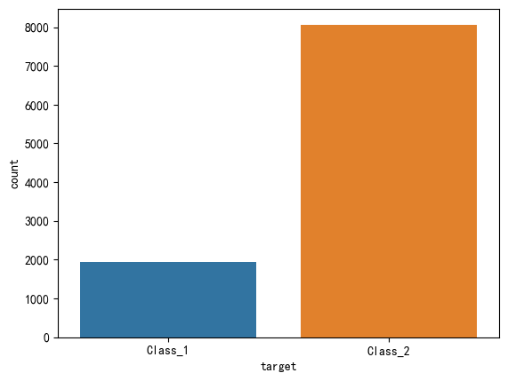

使用上面方式获取数据不可行,然后使用随机欠采样获取响应的数据

随机欠采样获取数据

#随机欠采样获取数据
# 首先获取纯净的x和y
y=data['target']
x=data.drop(['id','target'],axis=1)
y.shape,x.shape#((61878,), (61878, 93))

x.head()

	feat_1	feat_4	feat_5	feat_6	feat_7	feat_8	feat_10	...	feat_84	feat_85	feat_86	feat_87	feat_90
0	1	0	0	0	0	0	0	...	0	1	0	0	0
1	0	0	0	0	0	1	0	...	0	0	0	0	0
2	0	0	0	0	0	1	0	...	0	0	0	0	0
3	1	1	6	1	5	0	1	...	22	0	1	2	0
4	0	0	0	0	0	0	0	...	0	1	0	0	1

y.head()

0    Class_1
1    Class_1
2    Class_1
3    Class_1
4    Class_1
Name: target, dtype: object

# 随机欠采样
from imblearn.under_sampling import RandomUnderSampler
ran=RandomUnderSampler(random_state=66)
ran_x,ran_y=ran.fit_resample(x,y)
ran_x.shape,ran_y.shape#((17361, 93), (17361,))

# 欠采样后查看数据分布
sns.countplot(x=ran_y,hue=ran_y)
plt.show()

标签值转换为数字

ran_y.head()

0    Class_1
1    Class_1
2    Class_1
3    Class_1
4    Class_1
Name: target, dtype: object

from sklearn.preprocessing import LabelEncoder
le= LabelEncoder()
num_y=le.fit_transform(ran_y)

array([0, 0, 0, ..., 8, 8, 8])

数据分割

# 分割数据
from sklearn.model_selection import train_test_split
x_train,x_test,y_train,y_test=train_test_split(ran_x,num_y,random_state=6,test_size=0.2)

模型训练

# 模型训练
from sklearn.ensemble import RandomForestClassifier
rfc=RandomForestClassifier(random_state=66,oob_score=True)
rfc.fit(x_train,y_train)

模型评估

# 模型评估
pre=rfc.predict(x_test)
score=rfc.score(x_test,y_test)
print("score:",score)#score: 0.7745465015836452

pre

array([6, 6, 6, ..., 7, 5, 4])

# 图形化查看预测结果数据分布
sns.countplot(x=pre)
plt.tight_layout()
plt.show()

# 按照比赛评分标准评估模型
from sklearn.metrics import log_loss
from sklearn.preprocessing import OneHotEncoder
#log_loss方法输入参数必须是onehot编码的所以对输入值做如下转换：
he=OneHotEncoder(sparse_output=False)
hot_pre=he.fit_transform(pre.reshape(-1,1))
hot_y_test=he.fit_transform(y_test.reshape(-1,1))

hot_pre

array([[0., 0., 0., ..., 1., 0., 0.],
       [0., 0., 0., ..., 1., 0., 0.],
       [0., 0., 0., ..., 1., 0., 0.],
       ...,
       [0., 0., 0., ..., 0., 1., 0.],
       [0., 0., 0., ..., 0., 0., 0.],
       [0., 0., 0., ..., 0., 0., 0.]])

logscore=log_loss(hot_y_test,hot_pre,normalize=True)
print("多分类对数损失logscore:",logscore)#多分类对数损失logscore: 8.126167752282964
'''
说明，根据logloss计算公式可知，更准确真实的结果应该是模型预测属于某一类的概率取对数之和，而上面的hot_pre预测值只有0和1的最终结果，（所有的0，在预测错的情况下，都会取1e-15次方，导致log值极大，导致最终结果偏大）所以上面的多分类对数损失logscore: 8.126167752282964，应该使用预测概率来计算
'''

#使用模型预测并以概率形式返回预测结果
pre_pro=rfc.predict_proba(x_test)
pre_pro
#predict_proba的返回结果形式正好就是矩阵形式，因此我们不需要onehot编码了：

array([[0.14, 0.2 , 0.09, ..., 0.22, 0.06, 0.05],
       [0.06, 0.09, 0.06, ..., 0.52, 0.04, 0.12],
       [0.08, 0.08, 0.13, ..., 0.5 , 0.04, 0.06],
       ...,
       [0.05, 0.  , 0.  , ..., 0.  , 0.89, 0.02],
       [0.11, 0.04, 0.04, ..., 0.06, 0.18, 0.06],
       [0.  , 0.  , 0.  , ..., 0.  , 0.  , 0.  ]])

logscore=log_loss(hot_y_test,pre_pro,normalize=True)
print("多分类对数损失logscore:",logscore)#多分类对数损失logscore: 0.7482532726303186，相比直接使用0-1结果明显减小了

模型调优

我们对随机森林api这几个超参数逐一调优，并可视化观察模型表现：

n_estimators, max_feature, max_depth, min_samples_leaf

注意，实际工作中我们可能会使用交叉验证网格搜索GridSearchCV来进行超参数调优，我们现在手动调优是为了加深对模型调优的理解。

树⽊数量n_estimators

# 模型训练
import numpy as np
parames=np.arange(30,500,20)
scores=np.zeros(len(parames))
logscores=np.zeros(len(parames))
for i,param in enumerate(parames):
    rfc1=RandomForestClassifier(random_state=66,
                            oob_score=True,
                            n_estimators=param,
                            max_depth=10, 
                            max_features=10, 
                            min_samples_leaf=10, 
                            n_jobs=-1)
    rfc1.fit(x_train,y_train)
    scores[i]=rfc1.oob_score_
    pre_proba=rfc1.predict_proba(x_test)
    logscores[i]=log_loss(y_test,pre_proba, normalize=True)

plt.figure(figsize=(20,6),dpi=100)
plt.subplot(1,2,1)
plt.plot(parames,logscores)
plt.title("多分类对数损失")
plt.xlabel("n_estimators")
plt.ylabel("多分类对数损失值")
plt.grid()
plt.subplot(1,2,2)
plt.plot(parames,scores)
plt.title("模型得分")
plt.xlabel("n_estimators")
plt.ylabel("模型包外得分")
plt.grid()
plt.show()

经过图像展示,最后确定n_estimators=400的时候,表现效果不错

最大树深度max_depth

# 模型训练
import numpy as np
parames=np.arange(1,100,5)
scores=np.zeros(len(parames))
logscores=np.zeros(len(parames))
for i,param in enumerate(parames):
    rfc2=RandomForestClassifier(random_state=66,
                            oob_score=True,
                            n_estimators=400,
                            max_depth=param, 
                            max_features=10, 
                            min_samples_leaf=10, 
                            n_jobs=-1)
    rfc2.fit(x_train,y_train)
    scores[i]=rfc2.oob_score_
    pre_proba=rfc2.predict_proba(x_test)
    logscores[i]=log_loss(y_test,pre_proba, normalize=True)
    plt.figure(figsize=(20,6),dpi=100)
plt.subplot(1,2,1)
plt.plot(parames,logscores)
plt.title("多分类对数损失")
plt.xlabel("max_depth")
plt.ylabel("多分类对数损失值")
plt.grid()
plt.subplot(1,2,2)
plt.plot(parames,scores)
plt.title("模型得分")
plt.xlabel("max_depth")
plt.ylabel("模型包外得分")
plt.grid()
plt.show()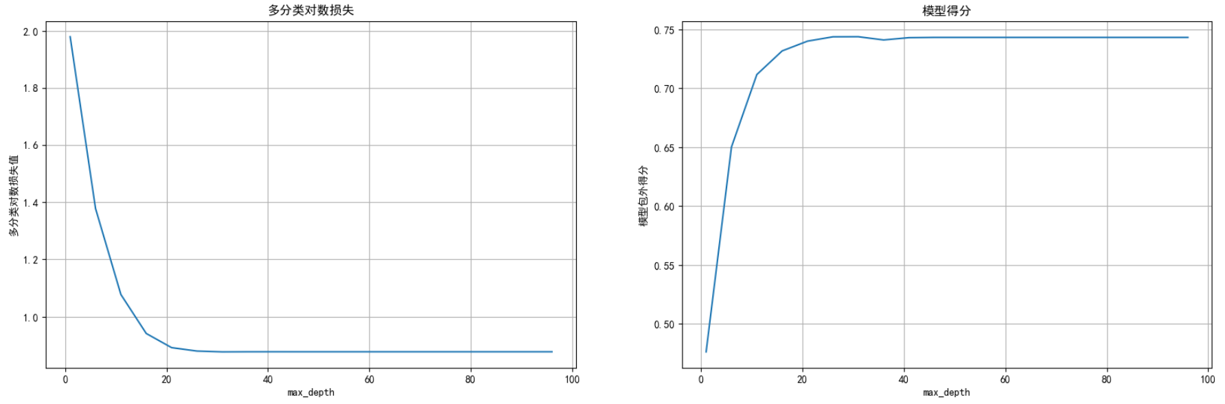

从上图得出最大树深度在20左右模型表现最好

决策树的最⼤特征数量max_features

# 模型训练
import numpy as np
parames=np.arange(1,25,5)
scores=np.zeros(len(parames))
logscores=np.zeros(len(parames))
for i,param in enumerate(parames):
    rfc3=RandomForestClassifier(random_state=66,
                            oob_score=True,
                            n_estimators=400,
                            max_depth=20, 
                            max_features=param, 
                            min_samples_leaf=10, 
                            n_jobs=-1)
    rfc3.fit(x_train,y_train)
    scores[i]=rfc3.oob_score_
    pre_proba=rfc3.predict_proba(x_test)
    logscores[i]=log_loss(y_test,pre_proba, normalize=True)
    plt.figure(figsize=(20,6),dpi=100)
plt.subplot(1,2,1)
plt.plot(parames,logscores)
plt.title("多分类对数损失")
plt.xlabel("max_features")
plt.ylabel("多分类对数损失值")
plt.grid()
plt.subplot(1,2,2)
plt.plot(parames,scores)
plt.title("模型得分")
plt.xlabel("max_features")
plt.ylabel("模型包外得分")
plt.grid()
plt.show()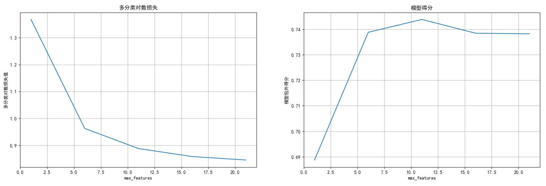

每个决策树的最⼤特征数量为12时模型性能最好

叶⼦节点的最⼩样本数min_samples_leaf

# 模型训练
import numpy as np
parames=np.arange(1,800,30)
scores=np.zeros(len(parames))
logscores=np.zeros(len(parames))
for i,param in enumerate(parames):
    rfc4=RandomForestClassifier(random_state=66,
                            oob_score=True,
                            n_estimators=400,
                            max_depth=20, 
                            max_features=12, 
                            min_samples_leaf=param, 
                            n_jobs=-1)
    rfc4.fit(x_train,y_train)
    scores[i]=rfc4.oob_score_
    pre_proba=rfc4.predict_proba(x_test)
    logscores[i]=log_loss(y_test,pre_proba, normalize=True)
    plt.figure(figsize=(20,6),dpi=100)
plt.subplot(1,2,1)
plt.plot(parames,logscores)
plt.title("多分类对数损失")
plt.xlabel("min_samples_leaf")
plt.ylabel("多分类对数损失值")
plt.grid()
plt.subplot(1,2,2)
plt.plot(parames,scores)
plt.title("模型得分")
plt.xlabel("min_samples_leaf")
plt.ylabel("模型包外得分")
plt.grid()
plt.show()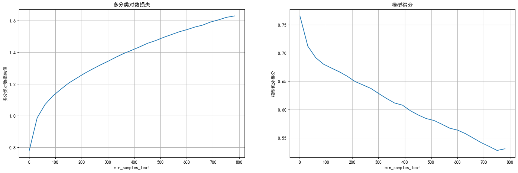

叶⼦节点的最⼩样本数为1时模型表现最好

最优参数训练模型

# 模型训练
rfc5=RandomForestClassifier(random_state=66,
                        oob_score=True,
                        n_estimators=400,
                        max_depth=20, 
                        max_features=12, 
                        min_samples_leaf=1, 
                        n_jobs=-1)
rfc5.fit(x_train,y_train)
score=rfc5.oob_score_
pre_proba=rfc5.predict_proba(x_test)
logscores=log_loss(y_test,pre_proba, normalize=True)
print(f'oobscoer:{score}\nlogscores:{logscores}')

oobscoer:0.7716733870967742
logscores:0.7166710553193704
# 调优之前：
# oobscore: 0.7611607142857143
# logscore: 0.7482532726303186
'''
从上面结果可以看出，超参数调优并非那么简单，很多时候，数据的重新切分，参数调优顺序都可能影响最终结果，所以，我们仅仅直到调优的过程即可
'''

生成提交数据

# 获取测试数据
test_data=pd.read_csv(r"D:\learn\000人工智能数据大全\经典数据集\奥托集团产品分类挑战赛\test.csv")
test_data.head()

	id	feat_1	feat_2	feat_3	feat_4	feat_7	feat_8	...	feat_85	feat_86	feat_87	feat_88	feat_89	feat_91	feat_92	feat_93
0	1	0	0	0	0	0	0	...	0	11	1	20	0	0	0	0
1	2	2	2	14	16	0	0	...	0	0	0	0	4	0	2	0
2	3	0	1	12	1	0	0	...	0	0	0	2	0	0	0	1
3	4	0	0	0	1	0	0	...	3	1	0	0	0	0	0	0
4	5	1	0	0	1	1	2	...	0	0	0	0	0	9	0	0

test_data_dropid=test_data.drop('id',axis=1)
test_data_dropid.head()

	feat_1	feat_2	feat_3	feat_4	feat_7	feat_8	feat_10	...	feat_85	feat_86	feat_87	feat_88	feat_89	feat_91	feat_92	feat_93
0	0	0	0	0	0	0	3	...	0	11	1	20	0	0	0	0
1	2	2	14	16	0	0	0	...	0	0	0	0	4	0	2	0
2	0	1	12	1	0	0	0	...	0	0	0	2	0	0	0	1
3	0	0	0	1	0	0	0	...	3	1	0	0	0	0	0	0
4	1	0	0	1	1	2	3	...	0	0	0	0	0	9	0	0

res=rfc5.predict_proba(test_data_dropid)
res

array([[0.00867396, 0.07792025, 0.21167363, ..., 0.05370235, 0.01041452,
        0.00655165],
       [0.05561672, 0.04926894, 0.03698527, ..., 0.02817363, 0.31065767,
        0.03571542],
       [0.0075    , 0.005     , 0.0025    , ..., 0.00266667, 0.02705556,
        0.00561111],
       ...,
       [0.02069945, 0.29311995, 0.30004326, ..., 0.05345355, 0.01400344,
        0.0080886 ],
       [0.00557086, 0.36087861, 0.11366321, ..., 0.01720327, 0.00135527,
        0.00459146],
       [0.0348605 , 0.17931501, 0.31182602, ..., 0.17517756, 0.01515248,
        0.01724063]])

 res.shape#(144368, 9)

#按照比赛要求整理列名
resdata=pd.DataFrame(res,columns=['Class_'+str(i) for i in range(1,10)])
resdata.head()

#插入id列
resdata.insert(loc=0,column='id',value=test_data.id)
resdata.head()

id	Class_1	Class_2	Class_3	Class_4	Class_5	Class_6	Class_7	Class_8	Class_9
0	1	0.008674	0.077920	0.211674	0.622969	0.005850	0.002245	0.053702	0.010415	0.006552
1	2	0.055617	0.049269	0.036985	0.038553	0.018773	0.426257	0.028174	0.310658	0.035715
2	3	0.007500	0.005000	0.002500	0.002833	0.000000	0.946833	0.002667	0.027056	0.005611
3	4	0.028859	0.307226	0.270988	0.215828	0.001105	0.003443	0.022041	0.014304	0.136206
4	5	0.235738	0.011673	0.003789	0.002674	0.006961	0.024948	0.042312	0.266285	0.405619

#导出数据
resdata.to_csv(r"D:\learn\000人工智能数据大全\经典数据集\奥托集团产品分类挑战赛\lzssub.csv",index=False)

提交参赛数据

posted @ 2025-06-06 09:16 指尖下的世界阅读(40) 评论(0) 收藏举报

刷新页面返回顶部

	feat_1	feat_4	feat_5	feat_6	feat_7	feat_8	feat_10	...	feat_84	feat_85	feat_86	feat_87	feat_90
0	1	0	0	0	0	0	0	...	0	1	0	0	0
1	0	0	0	0	0	1	0	...	0	0	0	0	0
2	0	0	0	0	0	1	0	...	0	0	0	0	0
3	1	1	6	1	5	0	1	...	22	0	1	2	0
4	0	0	0	0	0	0	0	...	0	1	0	0	1

	id	feat_1	feat_2	feat_3	feat_4	feat_7	feat_8	...	feat_85	feat_86	feat_87	feat_88	feat_89	feat_91	feat_92	feat_93
0	1	0	0	0	0	0	0	...	0	11	1	20	0	0	0	0
1	2	2	2	14	16	0	0	...	0	0	0	0	4	0	2	0
2	3	0	1	12	1	0	0	...	0	0	0	2	0	0	0	1
3	4	0	0	0	1	0	0	...	3	1	0	0	0	0	0	0
4	5	1	0	0	1	1	2	...	0	0	0	0	0	9	0	0

	feat_1	feat_2	feat_3	feat_4	feat_7	feat_8	feat_10	...	feat_85	feat_86	feat_87	feat_88	feat_89	feat_91	feat_92	feat_93
0	0	0	0	0	0	0	3	...	0	11	1	20	0	0	0	0
1	2	2	14	16	0	0	0	...	0	0	0	0	4	0	2	0
2	0	1	12	1	0	0	0	...	0	0	0	2	0	0	0	1
3	0	0	0	1	0	0	0	...	3	1	0	0	0	0	0	0
4	1	0	0	1	1	2	3	...	0	0	0	0	0	9	0	0

	feat_1	feat_4	feat_5	feat_6	feat_7	feat_8	feat_10	...	feat_84	feat_85	feat_86	feat_87	feat_90
0	1	0	0	0	0	0	0	...	0	1	0	0	0
1	0	0	0	0	0	1	0	...	0	0	0	0	0
2	0	0	0	0	0	1	0	...	0	0	0	0	0
3	1	1	6	1	5	0	1	...	22	0	1	2	0
4	0	0	0	0	0	0	0	...	0	1	0	0	1

	id	feat_1	feat_2	feat_3	feat_4	feat_7	feat_8	...	feat_85	feat_86	feat_87	feat_88	feat_89	feat_91	feat_92	feat_93
0	1	0	0	0	0	0	0	...	0	11	1	20	0	0	0	0
1	2	2	2	14	16	0	0	...	0	0	0	0	4	0	2	0
2	3	0	1	12	1	0	0	...	0	0	0	2	0	0	0	1
3	4	0	0	0	1	0	0	...	3	1	0	0	0	0	0	0
4	5	1	0	0	1	1	2	...	0	0	0	0	0	9	0	0

	feat_1	feat_2	feat_3	feat_4	feat_7	feat_8	feat_10	...	feat_85	feat_86	feat_87	feat_88	feat_89	feat_91	feat_92	feat_93
0	0	0	0	0	0	0	3	...	0	11	1	20	0	0	0	0
1	2	2	14	16	0	0	0	...	0	0	0	0	4	0	2	0
2	0	1	12	1	0	0	0	...	0	0	0	2	0	0	0	1
3	0	0	0	1	0	0	0	...	3	1	0	0	0	0	0	0
4	1	0	0	1	1	2	3	...	0	0	0	0	0	9	0	0

指尖下的世界

今日事今日毕,今日无事早休息.