具有神经网络思维的Logistic回归
使用Numpy的基础Python、logistic回归
import torch
import numpy as np
import torch.nn as nn
import torch.nn.functional as F
import torch.optim as optim
from torchvision import datasets, transforms

import math
Part 1:Python Basics with Numpy
1 - Building basic functions with numpy
1.1 - sigmoid function, np.exp()
Exercise: Build a function that returns the sigmoid of a real number x. Use math.exp(x) for the exponential function.
def sig_function(x):
    s = 1.0 / (1 + 1/math.exp(x))
    return s
sig_function(3)
0.9525741268224334
Exercise: Implement the sigmoid function using numpy.
def sig_function_by_np(x):
    s = 1.0 / (1 + 1/np.exp(x))
    return s
x = np.array([1, 2, 3])
sig_function_by_np(x)
array([0.73105858, 0.88079708, 0.95257413])
1.2 - Sigmoid gradient
Exercise: Implement the function sigmoid_grad() to compute the gradient of the sigmoid function with respect to its input x.
# 对sigmoid函数求导
def sigmoid_grad(x):
    s = 1.0 / (1 + 1/np.exp(x))
    ds = s * (1 - s)
    return ds
sigmoid_grad(x)
array([0.19661193, 0.10499359, 0.04517666])
1.3 - Reshaping arrays
Exercise: Implement image2vector() that takes an input of shape (length, height, 3) and returns a vector of shape (lengthheight3, 1).
def image2vector(image):
    v = image.reshape((image.shape[0] * image.shape[1] * image.shape[2], 1))
    return v
image = np.array([[[ 0.67826139,  0.29380381],
        [ 0.90714982,  0.52835647],
        [ 0.4215251 ,  0.45017551]],

       [[ 0.92814219,  0.96677647],
        [ 0.85304703,  0.52351845],
        [ 0.19981397,  0.27417313]],

       [[ 0.60659855,  0.00533165],
        [ 0.10820313,  0.49978937],
        [ 0.34144279,  0.94630077]]])

print ("image2vector(image) = " + str(image2vector(image)))
image2vector(image) = [[0.67826139]
 [0.29380381]
 [0.90714982]
 [0.52835647]
 [0.4215251 ]
 [0.45017551]
 [0.92814219]
 [0.96677647]
 [0.85304703]
 [0.52351845]
 [0.19981397]
 [0.27417313]
 [0.60659855]
 [0.00533165]
 [0.10820313]
 [0.49978937]
 [0.34144279]
 [0.94630077]]
1.4 - Normalizing rows
Exercise: Implement normalizeRows() to normalize the rows of a matrix.
np.linalg.norm(x, ord=None, axis=None, keepdims=False)
- axis=1表示按行向量处理;axis=0表示按列向量处理
- keepding:是否保持矩阵的二维特性
x = np.array([
    [0, 3, 4],
    [1, 6, 4]])
np.linalg.norm(x, ord=1, axis=1, keepdims=True)
array([[ 7.],
       [11.]])
def normalizeRows(x):
    x_norm = np.linalg.norm(x, axis=1, keepdims=True) # 计算每一行的长度
    return x / x_norm # 利用numpy的广播,用矩阵与列向量相除
normalizeRows(x)
array([[0.        , 0.6       , 0.8       ],
       [0.13736056, 0.82416338, 0.54944226]])
1.5 - Broadcasting and the softmax function
Exercise: Implement a softmax function using numpy.
def softmax(x):
    x_exp = np.exp(x)
    x_sum = np.sum(x_exp, axis=1, keepdims=True)
    s = x_exp / x_sum
    return s
x = np.array([
    [9, 2, 5, 0, 0],
    [7, 5, 0, 0 ,0]])
print("softmax(x) = " + str(softmax(x)))
softmax(x) = [[9.80897665e-01 8.94462891e-04 1.79657674e-02 1.21052389e-04
  1.21052389e-04]
 [8.78679856e-01 1.18916387e-01 8.01252314e-04 8.01252314e-04
  8.01252314e-04]]
2 - Vectorization
2.1 Implement the L1 and L2 loss functions
Exercise: Implement the numpy vectorized version of the L1 loss.
def L1(yhat, y):
    loss = np.sum(np.abs(y-yhat))
    return loss
yhat = np.array([.9, 0.2, 0.1, .4, .9])
y = np.array([1, 0, 0, 1, 1])
print("L1 = " + str(L1(yhat,y)))
L1 = 1.1
Exercise: Implement the numpy vectorized version of the L2 loss.
def L2(yhat, y):
    loss = np.sum(np.power((y-yhat),2))
    return loss
yhat = np.array([.9, 0.2, 0.1, .4, .9])
y = np.array([1, 0, 0, 1, 1])
print("L2 = " + str(L2(yhat,y)))
L2 = 0.43
Part 2: Logistic Regression with a Neural Network Mindset
Code
import numpy as np
import matplotlib.pyplot as plt
import h5py
import scipy
from PIL import Image
from scipy import ndimage
from lr_utils import load_dataset
2 - Overview of the Problem set
train_set_x_orig, train_set_y, test_set_x_orig, test_set_y, classes = load_dataset()
index = 25
plt.imshow(train_set_x_orig[index])
print ("y = " + str(train_set_y[:, index]) +
       ", it's a '" + classes[np.squeeze(train_set_y[:, index])].decode("utf-8") +  "' picture.")
y = [1], it's a 'cat' picture.

print(train_set_y.shape)
print(train_set_y[:,25]) # 相当与一维
print(np.squeeze(train_set_y[:,25]))
(1, 209)
[1]
1
classes[1].decode("utf-8")
'cat'
Exercise: Find the values for:
- m_train (number of training examples)
- m_test (number of test examples)
- num_px ( height and width of a training image)
Remember that train_set_x_orig is a numpy-array of shape (m_train, num_px, num_px, 3).
m_train = train_set_y.shape[1]
m_test = test_set_y.shape[1]
num_px = train_set_x_orig.shape[1]
print(m_train)
print(m_test)
print(num_px)
209
50
64
Exercise: Reshape the training and test data sets so that images of size (num_px, num_px, 3) are flattened into single vectors of shape.
列是训练集的样本数量:
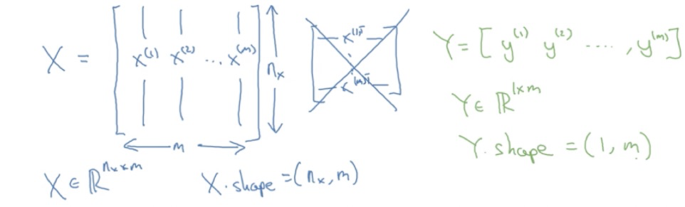
train_set_x_flatten = train_set_x_orig.reshape(train_set_x_orig.shape[1]*train_set_x_orig.shape[2]
                                               *train_set_x_orig.shape[3], train_set_x_orig.shape[0])
test_set_x_flatten = test_set_x_orig.reshape(m_test, -1).T # -1让程序帮忙算,最后程序算出来时12288列,最后用一个T表示转置

print ("train_set_x_flatten shape: " + str(train_set_x_flatten.shape))
print ("train_set_y shape: " + str(train_set_y.shape))
print ("test_set_x_flatten shape: " + str(test_set_x_flatten.shape))
print ("test_set_y shape: " + str(test_set_y.shape))
train_set_x_flatten shape: (12288, 209)
train_set_y shape: (1, 209)
test_set_x_flatten shape: (12288, 50)
test_set_y shape: (1, 50)
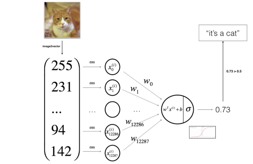
彩色图像的像素值实际上是从0到255范围内的三个数字的向量。机器学习中一个常见的预处理步骤是对数据集进行居中和标准化,这意味着可以减去每个示例中整个numpy数组的平均值,然后将每个示例除以整个numpy数组的标准偏差。但对于图片数据集,可以将数据集的每一行除以255(像素通道的最大值),因为在RGB中不存在比255大的数据,所以除以255让标准化的数据位于[0,1]之间,现在标准化我们的数据集:
train_set_x = train_set_x_flatten/255.
test_set_x = test_set_x_flatten/255.
3 - General Architecture of the learning algorithm
4 - Building the parts of our algorithm
Exercise: Using your code from “Python Basics”, implement sigmoid().
def sigmoid(z):
    s = 1 / (1 + np.exp(-z))
    return s
print ("sigmoid([0, 2]) = " + str(sigmoid(np.array([0,2]))))
sigmoid([0, 2]) = [0.5 0.88079708]
Exercise: Implement parameter initialization in the cell below.
def initialize_with_zeros(dim):
    """
    This function creates a vector of zeros of shape (dim, 1) for w and initializes b to 0.

    Argument:
    dim -- size of the w vector we want (or number of parameters in this case)

    Returns:
    w -- initialized vector of shape (dim, 1)
    b -- initialized scalar (corresponds to the bias)
    """
    w = np.zeros((dim, 1))
    b = 0

    # 使用断言来确保我要的数据是正确的
    assert(w.shape == (dim, 1)) # w的维度是(dim,1)
    assert(isinstance(b, float) or isinstance(b, int)) # b的类型是float或者是int

    return w, b
dim = 2
w, b = initialize_with_zeros(dim)
print ("w = " + str(w))
print ("b = " + str(b))
w = [[0.]
 [0.]]
b = 0
Exercise: Implement a function propagate() that computes the cost function and its gradient.
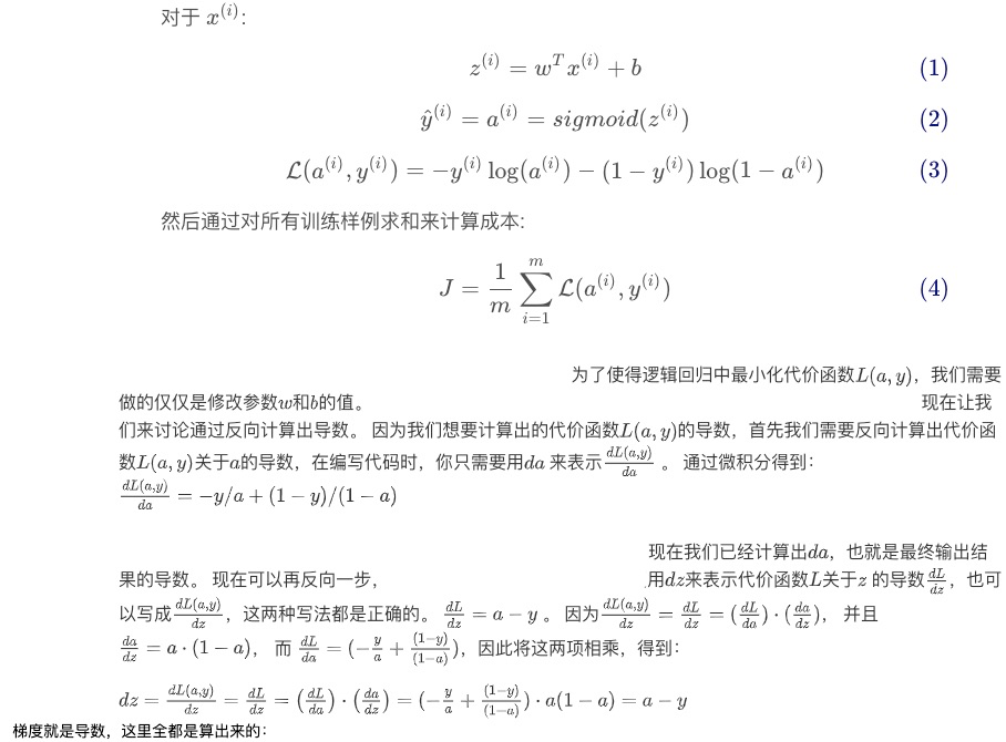
梯度就是导数,这里全都是算出来的:
def propagate(w, b, X, Y):
    """
    Implement the cost function and its gradient for the propagation explained above

    Arguments:
    w -- weights, a numpy array of size (num_px * num_px * 3, 1)
    b -- bias, a scalar
    X -- data of size (num_px * num_px * 3, number of examples)
    Y -- true "label" vector (containing 0 if non-cat, 1 if cat) of size (1, number of examples)

    Return:
    cost -- negative log-likelihood cost for logistic regression
    dw -- gradient of the loss with respect to w, thus same shape as w
    db -- gradient of the loss with respect to b, thus same shape as b

    """
    m = X.shape[1]
    A = sigmoid(np.dot(w.T, X) + b)
    cost = -(1/m) * np.sum(Y * np.log(A) + (1 - Y)*np.log(1 - A))

    dw = (1.0/m)*np.dot(X,(A-Y).T)
    db = (1.0/m)*np.sum(A-Y)


    assert(dw.shape == w.shape)
    assert(db.dtype == float)
    cost = np.squeeze(cost)
    assert(cost.shape == ())a

    grads = {"dw": dw,
             "db": db}

    return grads, cost
w, b, X, Y = np.array([[1.],[2.]]), 2., np.array([[1.,2.,-1.],[3.,4.,-3.2]]), np.array([[1,0,1]])
grads, cost = propagate(w, b, X, Y)
print ("dw = " + str(grads["dw"]))
print ("db = " + str(grads["db"]))
print ("cost = " + str(cost))
dw = [[0.99845601]
 [2.39507239]]
db = 0.001455578136784208
cost = 5.801545319394553
Exercise: Write down the optimization function.
def optimize(w, b, X, Y, num_iterations, learning_rate, print_cost = False):
    """
    This function optimizes w and b by running a gradient descent algorithm

    Arguments:
    w -- weights, a numpy array of size (num_px * num_px * 3, 1)
    b -- bias, a scalar
    X -- data of shape (num_px * num_px * 3, number of examples)
    Y -- true "label" vector (containing 0 if non-cat, 1 if cat), of shape (1, number of examples)
    num_iterations -- number of iterations of the optimization loop
    learning_rate -- learning rate of the gradient descent update rule
    print_cost -- True to print the loss every 100 steps

    Returns:
    params -- dictionary containing the weights w and bias b
    grads -- dictionary containing the gradients of the weights and bias with respect to the cost function
    costs -- list of all the costs computed during the optimization, this will be used to plot the learning curve.

    """
    costs = []
    for i in range(num_iterations):
        grads, cost = propagate(w, b, X, Y)

        dw = grads['dw']
        db = grads['db']

        w = w - dw*learning_rate
        b = b - db*learning_rate

        # Record the costs
        if i % 100 == 0:
            costs.append(cost)
        # Print the cost every 100 training examples
        if (print_cost) and (i % 100 == 0):
            print("迭代的次数: %i , 误差值: %f" % (i,cost))

    params = {'w':w, 'b':b}
    grads = {'dw':dw, 'db':db} # for循环不是一个函数体,所以for循环中的变量i的作用域其实和for循环同级
    """
    def foo():
      i=None
      for i in range(1,5,2):
        pass
      print(i)
    foo() # 结果为3,即循环结束i的最终值
    """
    return params, grads, costs
params, grads, costs = optimize(w, b, X, Y, num_iterations= 100, learning_rate = 0.009, print_cost = False)

print ("w = " + str(params["w"]))
print ("b = " + str(params["b"]))
print ("dw = " + str(grads["dw"]))
print ("db = " + str(grads["db"]))
w = [[0.19033591]
 [0.12259159]]
b = 1.9253598300845747
dw = [[0.67752042]
 [1.41625495]]
db = 0.21919450454067652
Exercise: The previous function will output the learned w and b. We are able to use w and b to predict the labels for a dataset X. Implement the predict() function.
def predict(w, b, X):
    '''
    Predict whether the label is 0 or 1 using learned logistic regression parameters (w, b)

    Arguments:
    w -- weights, a numpy array of size (num_px * num_px * 3, 1)
    b -- bias, a scalar
    X -- data of size (num_px * num_px * 3, number of examples)

    Returns:
    Y_prediction -- a numpy array (vector) containing all predictions (0/1) for the examples in X
    '''
    m = X.shape[1]
    Y_prediction = np.zeros((1, m))
    w = w.reshape(X.shape[0],1) # 确保维数正确?

    A = sigmoid(np.dot(w.T, X) + b)
    for i in range(A.shape[1]):
        if A[0, i] > 0.5:
            Y_prediction[0, i] = 1
        else:
            Y_prediction[0, i] = 0

    assert(Y_prediction.shape == (1, m))
    return Y_prediction
w = np.array([[0.1124579],[0.23106775]])
b = -0.3
X = np.array([[1.,-1.1,-3.2],[1.2,2.,0.1]])
print ("predictions = " + str(predict(w, b, X)))
predictions = [[1. 1. 0.]]
5 - Merge all functions into a model
Exercise: Implement the model function.
def model(X_train, Y_train, X_test, Y_test, num_iterations = 2000, learning_rate = 0.5, print_cost = False):
    """
    Builds the logistic regression model by calling the function you've implemented previously

    Arguments:
    X_train -- training set represented by a numpy array of shape (num_px * num_px * 3, m_train)
    Y_train -- training labels represented by a numpy array (vector) of shape (1, m_train)
    X_test -- test set represented by a numpy array of shape (num_px * num_px * 3, m_test)
    Y_test -- test labels represented by a numpy array (vector) of shape (1, m_test)
    num_iterations -- hyperparameter representing the number of iterations to optimize the parameters
    learning_rate -- hyperparameter representing the learning rate used in the update rule of optimize()
    print_cost -- Set to true to print the cost every 100 iterations

    Returns:
    d -- dictionary containing information about the model.
    """
    w, b = initialize_with_zeros(X_train.shape[0])
    parameters, grads, costs = optimize(w, b, X_train, Y_train, num_iterations, learning_rate, print_cost)

    w = parameters['w']
    b = parameters['b']

    Y_prediction_test = predict(w, b, X_test)
    Y_prediction_train = predict(w, b, X_train)

    print("train accuracy: {} %".format(100 - np.mean(np.abs(Y_prediction_train - Y_train)) * 100))
    print("test accuracy: {} %".format(100 - np.mean(np.abs(Y_prediction_test - Y_test)) * 100))

    d = {"costs": costs,
         "Y_prediction_test": Y_prediction_test,
         "Y_prediction_train" : Y_prediction_train,
         "w" : w,
         "b" : b,
         "learning_rate" : learning_rate,
         "num_iterations": num_iterations}
    return d
d = model(train_set_x, train_set_y, test_set_x, test_set_y,
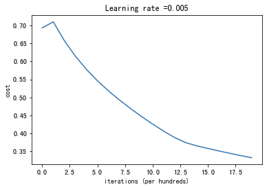
num_iterations = 2000, learning_rate = 0.005, print_cost = True)
迭代的次数: 0 , 误差值: 0.693147
迭代的次数: 100 , 误差值: 0.709726
迭代的次数: 200 , 误差值: 0.657712
迭代的次数: 300 , 误差值: 0.614611
迭代的次数: 400 , 误差值: 0.578001
迭代的次数: 500 , 误差值: 0.546372
迭代的次数: 600 , 误差值: 0.518331
迭代的次数: 700 , 误差值: 0.492852
迭代的次数: 800 , 误差值: 0.469259
迭代的次数: 900 , 误差值: 0.447139
迭代的次数: 1000 , 误差值: 0.426262
迭代的次数: 1100 , 误差值: 0.406617
迭代的次数: 1200 , 误差值: 0.388723
迭代的次数: 1300 , 误差值: 0.374678
迭代的次数: 1400 , 误差值: 0.365826
迭代的次数: 1500 , 误差值: 0.358532
迭代的次数: 1600 , 误差值: 0.351612
迭代的次数: 1700 , 误差值: 0.345012
迭代的次数: 1800 , 误差值: 0.338704
迭代的次数: 1900 , 误差值: 0.332664
train accuracy: 91.38755980861244 %
test accuracy: 34.0 %
costs = np.squeeze(d['costs'])
plt.plot(costs)
plt.ylabel('cost')
plt.xlabel('iterations (per hundreds)')
plt.title("Learning rate =" + str(d["learning_rate"]))
plt.show()
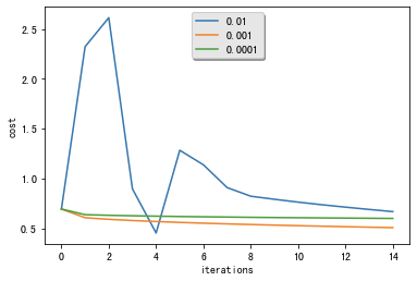
6 - Further analysis
learning_rates = [0.01, 0.001, 0.0001]
models = {}
for i in learning_rates:
    print ("learning rate is: " + str(i))
    models[str(i)] = model(train_set_x, train_set_y, test_set_x, test_set_y, num_iterations = 1500, learning_rate = i, print_cost = False)
    print ('\n' + "-------------------------------------------------------" + '\n')

for i in learning_rates:
    plt.plot(np.squeeze(models[str(i)]["costs"]), label= str(models[str(i)]["learning_rate"]))

plt.ylabel('cost')
plt.xlabel('iterations')

legend = plt.legend(loc='upper center', shadow=True)
frame = legend.get_frame()
frame.set_facecolor('0.90')
plt.show()
learning rate is: 0.01
train accuracy: 71.29186602870814 %
test accuracy: 74.0 %

-------------------------------------------------------

learning rate is: 0.001
train accuracy: 74.16267942583733 %
test accuracy: 34.0 %

-------------------------------------------------------

learning rate is: 0.0001
train accuracy: 66.02870813397129 %
test accuracy: 34.0 %

-------------------------------------------------------

 浙公网安备 33010602011771号