手写 k近邻 与 全连接神经网络 算法
KNN(K-近邻算法)
K-近邻算法的介绍
参考:
https://blog.csdn.net/weixin_39910711/article/details/114440816
手写knn算法,实现mnist的图片数字识别
# 手动 实现knn
import io
from struct import pack,unpack
import random
from PIL import Image
import time
import numpy as np
PIXEL = -1
WIDTH = -1
LEGTH = -1
def set_randon_seed(seed):
    random.seed(seed)

# 参考: https://yann.lecun.com/exdb/mnist/ parse mnist dataest
def read_pic(pic_num,label_path = "./mnist/train-labels.idx1-ubyte",images_path = "./mnist/train-images.idx3-ubyte"):
    global PIXEL,WIDTH,LENGTH
    fp_label = open(label_path,'rb')
    label_data = fp_label.read()
    io_label = io.BytesIO(label_data)

    fp_image = open(images_path,'rb')
    image_data = fp_image.read()
    io_image = io.BytesIO(image_data)

    assert 0x00000801 == unpack(">I",io_label.read(4))[0]
    assert 0x00000803 == unpack(">I",io_image.read(4))[0]
    all_size = unpack(">I",io_label.read(4))[0]
    io_image.read(4)
    dx = unpack(">I",io_image.read(4))[0]
    dy = unpack(">I",io_image.read(4))[0]
    PIXEL = dx * dy
    LENGTH = dx
    WIDTH = dy


    image_all = [io_image.read(PIXEL) for _ in range(all_size) ]
    labels_all = [io_label.read(1) for _ in range(all_size)]
    # random get pic
    random_list = random.sample(range(all_size), pic_num)

    image_list = []
    labels_list = []
    for i in random_list:
        image_list.append( list(image_all[i]))
        labels_list.append(labels_all[i][0])

    return image_list,labels_list


# 实际上,数据集提供的是二值图像,即灰白图片,0 代表白色,255 代表黑色,其他值介于0到255之间
def pt_image(image_list):
    image_np = np.array(image_list)
    two_dim_array = image_np.reshape(-1, WIDTH)
    image = Image.fromarray(two_dim_array.astype(np.uint8), mode='L')
    image.show()


def knn(k,train_dataset,train_labels,test_data):
    train_dataset_np = np.array(train_dataset)
    test_np = np.array(test_data)

    sub_np = np.sum((train_dataset_np - test_np) ** 2,axis=1) # axis=1:表示沿着 水平方向(列的方向)进行操作,也就是说,对每一行的数据进行操作。  axis=0:表示沿着 垂直方向(行的方向)进行操作,也就是说,对每一列的数据进行操作
    least_indices = np.argpartition(sub_np, k)[:k]          # 返回k个差值平方最小的元素的下标

    counter = np.zeros(15, dtype=int)
    for indice in least_indices:
        counter[train_labels[indice]] += 1

    idx = -1
    cnt = -1
    for i in range(len(counter)):
        val = counter[i]
        if val > cnt:
            cnt = val
            idx = i
    return idx


dataset_num = 20000
test_num = 200
set_randon_seed(0)
train_images,train_labels = read_pic(dataset_num)
test_images,test_labels = read_pic(test_num,label_path="./mnist/t10k-labels.idx1-ubyte",images_path="./mnist/t10k-images.idx3-ubyte")


# # 下面进行图片预测:
# test_k = [1,3,5,7]
# for kk in test_k:
#     k = kk
#     correct_num = 0
#     for i in range(test_num):
#         test_data = test_images[i]
#         test_label = test_labels[i]
#         get_test_label_by_knn = knn(k,train_images,train_labels,test_data)
#         if test_label == get_test_label_by_knn:
#             correct_num += 1

#     print(f"when k = {k}, the accuracy_rate is {correct_num / test_num}")


start = time.time()
k = 5
correct_num = 0
for i in range(test_num):
    test_data = test_images[i]
    test_label = test_labels[i]
    get_test_label_by_knn = knn(k,train_images,train_labels,test_data)
    if test_label == get_test_label_by_knn:
        correct_num += 1
end = time.time()
print(f"the costed times is {end - start}")
print(f"when k = {k}, the accuracy_rate is {correct_num / test_num}")


# when k = 1, the accuracy_rate is 0.945
# when k = 3, the accuracy_rate is 0.965
# when k = 5, the accuracy_rate is 0.97
# when k = 7, the accuracy_rate is 0.97
用 Skelarn 库 + KNN算法解决鸢尾花问题
参考:
https://www.cnblogs.com/listenfwind/p/10685192.html
https://doc.aidaxue.com/tensorflow-course/05-iris.html#_1-鸢尾花问题背景
# from sklearn.datasets import load_iris
# from sklearn.model_selection import cross_val_score
# import matplotlib.pyplot as plt
# from sklearn.neighbors import KNeighborsClassifier
# #读取鸢尾花数据集
# iris = load_iris()
# x = iris.data # 数据集中的特征部分赋值给变量 x,x 是一个包含150个样本和4个特征的二维数组。
# y = iris.target # 数据集中的标签部分赋值给变量 y,y 是一个包含150个样本标签的一维数组,标签有3种不同的值(表示3个类别)。
# k_range = range(1, 31)
# k_error = []
# #循环,取k=1到k=31,查看误差效果
# for k in k_range:
# knn = KNeighborsClassifier(n_neighbors=k)
# #cv参数决定数据集划分比例,这里是按照5:1划分训练集和测试集
# scores = cross_val_score(knn, x, y, cv=6, scoring='accuracy') # 用于执行交叉验证。它将数据集划分为训练集和测试集,并计算模型在测试集上的得分。
# k_error.append(1 - scores.mean())
# #画图,x轴为k值,y值为误差值
# plt.plot(k_range, k_error)
# plt.xlabel('Value of K for KNN')
# plt.ylabel('Error')
# plt.show()
# 这里通过找误差最小的点,算出了 k的最佳取值
# 下面这个代码实际上就是: 通过sklearn自带的鸢尾花数据集,通过提取器
import matplotlib.pyplot as plt
import numpy as np
from matplotlib.colors import ListedColormap
from sklearn import neighbors, datasets
n_neighbors = 11
iris = datasets.load_iris()
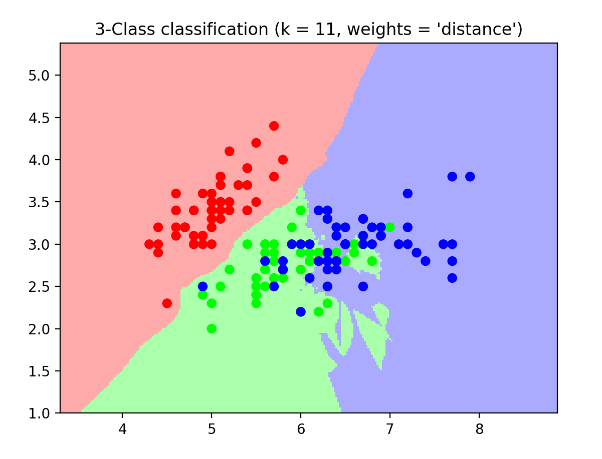
x = iris.data[:, :2] # 我们只采用前两个feature,方便画图在二维平面显示 , 花萼长度、花萼宽度、花瓣长度、花瓣宽度
y = iris.target
h = .02 # 网格中的步长
# 创建彩色的图
cmap_light = ListedColormap(['#FFAAAA', '#AAFFAA', '#AAAAFF'])
cmap_bold = ListedColormap(['#FF0000', '#00FF00', '#0000FF'])
#weights是KNN模型中的一个参数,上述参数介绍中有介绍,这里绘制两种权重参数下KNN的效果图
for weights in ['uniform', 'distance']:
# 创建了一个knn分类器的实例,并拟合数据。
clf = neighbors.KNeighborsClassifier(n_neighbors, weights=weights)
clf.fit(x, y)
# 绘制决策边界。为此,我们将为每个分配一个颜色
# 来绘制网格中的点 [x_min, x_max]x[y_min, y_max].
x_min, x_max = x[:, 0].min() - 1, x[:, 0].max() + 1
y_min, y_max = x[:, 1].min() - 1, x[:, 1].max() + 1
xx, yy = np.meshgrid(np.arange(x_min, x_max, h),
np.arange(y_min, y_max, h))
Z = clf.predict(np.c_[xx.ravel(), yy.ravel()])
# 将结果放入一个彩色图中
Z = Z.reshape(xx.shape)
plt.figure()
plt.pcolormesh(xx, yy, Z, cmap=cmap_light)
# 绘制训练点
plt.scatter(x[:, 0], x[:, 1], c=y, cmap=cmap_bold)
plt.xlim(xx.min(), xx.max())
plt.ylim(yy.min(), yy.max())
plt.title("3-Class classification (k = %i, weights = '%s')"
% (n_neighbors, weights))
plt.show()
绘制的二维图如下:
全连接神经网络
概念介绍
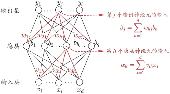
- 神经网络包括输入层、隐藏层和输出层,一个DNN结构只有一个输入层,一个输出层,输入层和输出层之间的都是隐藏层,隐藏层可能有好几层,隐藏层比较多(>2)的神经网络叫做深度神经网络(DNN的网络层数不包括输入层)。
- 每一层神经网络有若干神经元,层与层之间神经元相互连接,层内神经元互不连接,而且下一层每一个神经元连接上一层所有的神经元。
加权求和公式
- \(x_i^{l-1}\) 代表第
l-1层的第j个神经元的输入值。 - \(w_j^{l-1}\) 代表权重,即代表第
l-1层的第j个神经元到第l层的第i个神经元的权重。 - \(b_i^l\) 代表偏置值(bias),第
l层第i个神经元的偏置值。 - \(y_i^l\) 表示第
l层的第i个神经元接收到的上一层神经元的加权和。
激活函数
激活函数的功能:
- 激活函数给神经元引入了非线性的因素,使得神经网络可以逼近任何非线性函数,不仅限于线性模型。
- 激活函数通过 决定是否激活神经元(即神经元是否发出信号并继续传播),让神经网络能够进行 非线性变换,从而使网络具备处理复杂问题的能力。
常见的激活函数有这几类:
参考讲解: https://brickexperts.github.io/2019/09/03/激活函数/
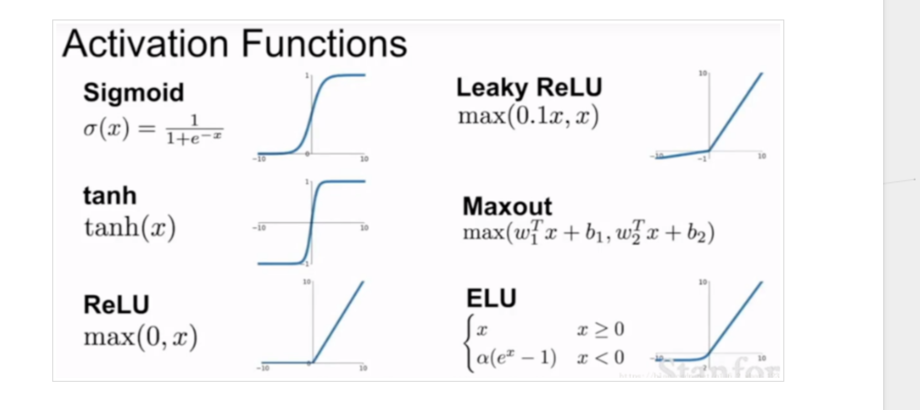
softmax激活函数
-
Softmax 是一种特定类型的激活函数,它通常用于神经网络的 输出层,尤其是在 多分类问题中,用于将网络的原始输出(logits)转换为概率分布。
-
Softmax 的主要功能是将神经网络的 输出层 的原始得分(logits)转化为 概率分布,并进行 多类分类。它的输出值表示每个类别的预测概率,所有类别的概率之和为 1,适用于多分类问题。
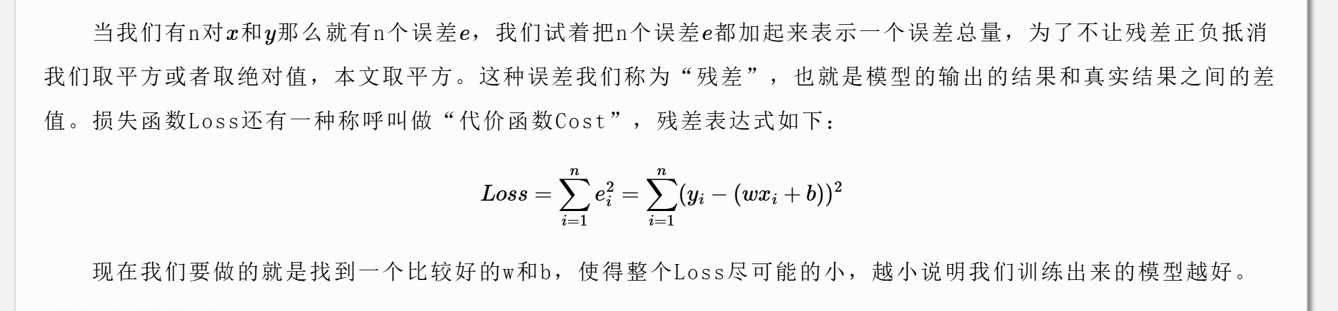
损失函数
反向传播算法(BP)
bp算法主要有以下三个步骤
- 前向计算每个神经元的输出值;
- 反向计算每个神经元的误差项e值;
- 最后用随机梯度下降算法迭代更新权重w和b。
这里求w和b用到了梯度下降算法,看这篇文章就行:
https://www.cnblogs.com/LXP-Never/p/9979207.html
学习率
学习率与梯度下降算法密切相关
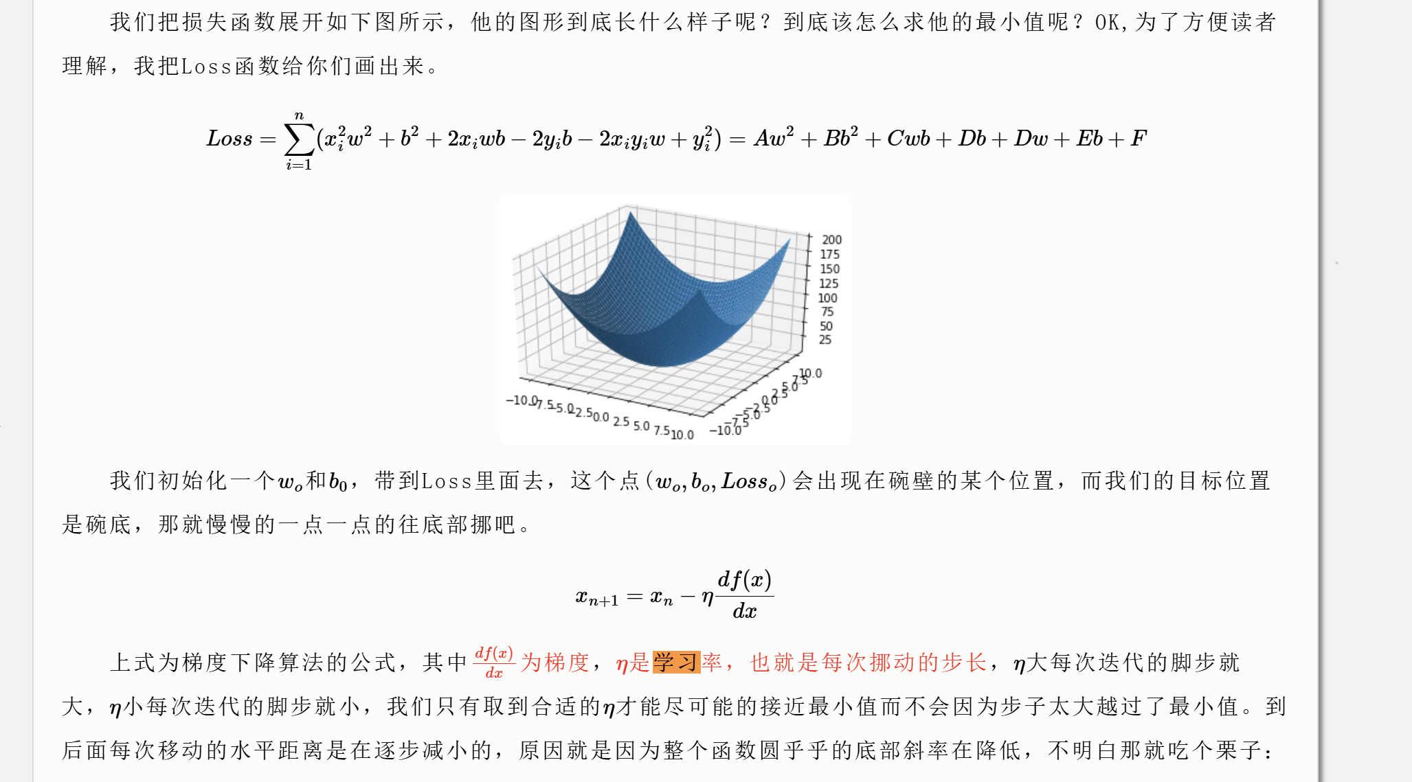
如上图,η是学习率,也就是每次挪动的步长。
-
梯度下降会计算损失函数对当前参数的梯度(即损失函数在当前参数位置的变化率),然后按照这个梯度的方向更新参数。学习率就控制着步长的大小。
-
通过多次迭代,不断调整w、b参数,最终使损失函数尽可能小,达到收敛。
-
学习率过大:如果学习率设置得过大,那么每次更新时步伐过大,可能会导致更新过程“跳跃”得太远,错过了损失函数的最小值,甚至会导致训练过程不收敛或者震荡。
-
学习率过小:如果学习率过小,更新的步伐会非常小,训练过程虽然稳定,但可能会非常缓慢,甚至在训练时间内无法收敛到一个好的解。
我对于全连接神经网络的理解
这里以 28x28 像素的数字图像识别为例
-
首先是图片识别神经网络的训练
-
我们会把0~9这10个数字用
One-hot编码来表示,比如说我们比较10个数字,那一个编码就是单位为10的列表,0可能被表示为: [1,0,0,0,0,0,0,0,0,0],1可能被表示为: [0,1,0,0,0,0,0,0,0,0] 等等使用One_Hot编码的优点如下:
-
避免模型将类别视为连续值。
-
使用 One-Hot 编码使得这些损失函数能够准确计算预测概率与真实标签之间的差距,从而有效指导模型的训练。
-
-
初始化 w、b的值。神经网络层数越多,用到的w、b的值也就越多,初始化的值也就越多。
-
设置好训练次数/轮数与学习率
较高的学习率意味着每次权重更新的步伐较大,较低的学习率则意味着步伐较小。学习率过大或过小都不合适。
-
开始训练
以一轮训练为例
-
把784个像素点作为x输入,从输入层到隐藏层,每个节点都需要经过加权函数,加权函数计算后会通过激活函数决定是否激活神经元。激活函数的输出,我们即为 z
-
之后我们把z作为输入,从隐藏层到更深的隐藏层进行传播,同样,每个z/节点都要经过加权函数,之后经过激活函数...
-
以此类推,一直到最后一轮,最后一轮是从隐藏层到输出层,实际上这一层一般只经过加权函数,不经过激活函数,或者经过Softmax激活函数。
-
最后,我们需要求输出与实际结果的均方差,之后根据梯度下降算法,求出w、b的梯度,并且更新一下w、b的值:
\(new\_w = w + 学习率 * 梯度\)
再下一轮训练开始前,new_w、new_b会作为 w,b参与下一轮的加权运算,以此类推,每轮训练都会更新一次 w、b的值,更新的次数就是训练的轮数!
另外,我们训练的过程中,是60000张图片同时训练,也就是说,每张图片在运算过程中用到的w、b值是相同的。
-
-
-
下面讲解如何进行图片识别
假设我们之前训练的神经网络模型有k层
- 把一张图片的所有像素点放入输入端,也就是有784个x
- 之后各个x经过了加权求和函数的计算,被送入了隐藏层,此时隐藏层会使用激活函数决定是否激活神经元。激活函数的值是z。
- 把z作为x进入下一层神经网络。。。以此类推 k 次(第k次不经过激活函数处理)。
- 最后一层应该有10个节点,通过计算这10个节点那个权重大,或者哪那个值,即可推断出最有可能的数字。
- ps:
- 对于某个数字图片而言,他在加权的过程中,一定会有若干条权值很高的神经网络传播线路,也一定会有权值很低的神经网络传播线路,越高的权值,代表它越匹配,越低的权值,代表他越不匹配。
- 而且对于这张图片的像素点而而言,一定有一些像素点对应的权值非常高,也一定有一些像素点对应的权值非常低,就像这张图片的特征似的,越能代表图片特征的像素点,其对应的权值就越高,反之,则会低一些。最后,根据权值计算出的是概率,概率最高的就是匹配的数字。
使用 tensorflow 库实现全连接神经网络识别 mnist图片
这里实现了四层全连接神经网络
import tensorflow as tf
from tensorflow import keras
from tensorflow.keras import datasets
import numpy as np
import matplotlib.pyplot as plt
import time


# 读取数据集
(x, y), (x_val, y_val) = datasets.mnist.load_data() # (x, y):训练集的数据和标签 (x_val, y_val):测试集的数据和标签
# 转换成浮点型张量,并映射到[-1, 1]区间,======> 这是因为许多神经网络在训练时,使用[-1, 1]的输入数据能够加速收敛,提高训练效率。
x = 2 * tf.convert_to_tensor(x, dtype=tf.float32) / 255. - 1
# 转换成整型张量    =======>    标签数据需要是整数类型、One-hot 编码前需要整数标签
y = tf.convert_to_tensor(y, dtype=tf.int32)
# one-hot编码
y = tf.one_hot(y, depth=10)
# 改变视图  [b, 28, 28]  =>  [b, 28*28]
x = tf.reshape(x, [-1, 28*28])

# 首先创建每个非线性层的W和b张量参数
# 每层的张量都需要被优化,故使用Variable类型,并使用截断的正态分布初始化权值张量
# 偏置向量初始化为0即可
# 第一层的参数
w1 = tf.Variable(tf.random.truncated_normal([784, 256], stddev=0.1))        # ====> w的值通过截断正态分布随机初始化,截断正态分布是通过从正态分布中采样,但将那些超过两倍标准差(stddev=0.1)的值裁剪掉,以避免极端值对训练造成影响。
b1 = tf.Variable(tf.zeros([256]))
# 第二层的参数
w2 = tf.Variable(tf.random.truncated_normal([256, 128], stddev=0.1))
b2 = tf.Variable(tf.zeros(128))
# 第三层的参数
w3 = tf.Variable(tf.random.truncated_normal([128, 10], stddev=0.1))
b3 = tf.Variable(tf.zeros([10]))


# 设置训练次数epochs及学习率lr
epochs = 100
lr = 0.01                       # ===》 它控制模型更新参数的速度。较高的学习率意味着每次权重更新的步伐较大,较低的学习率则意味着步伐较小。lr=0.01 是一个常见的学习率,用来平衡更新速度和模型收敛的稳定性。
# 记录每次的损失
list_loss = np.zeros([epochs])  # ===》 初始化一个长度为 epochs 的数组,用于记录每一轮训练结束后的损失值。
list_epoch = np.arange(epochs)


start = time.time()

for epoch in range(epochs):
    with tf.GradientTape() as tape:  # 构建梯度记录环境
        # 第一层计算 [b, 784]@[784, 256]+[256] => [b, 256]+[256] => [b,256]+[b, 256]
        h1 = x@w1 + tf.broadcast_to(b1, [x.shape[0], 256])          # ===> 计算: x*w1 + b1
        h1 = tf.nn.relu(h1)  # 通过激活函数                          # ===> 通过relu激活函数!
        # 第二层计算 [b, 256] => [b, 128]
        h2 = h1@w2 + b2
        h2 = tf.nn.relu(h2)
        # 输出层计算 [b, 128] => [b, 10]
        out = h2@w3 + b3                                            # ===> 第三层,同样计算 x*w3 + b3
        # print(out)
        # 计算y与out的均方差
        # print(tf.reduce_max(out))
        loss = tf.square(y - out)                                   # 计算方程,实际上就是损失函数
        loss = tf.reduce_mean(loss)                                 # 计算均方差
        list_loss[epoch] = loss
        # 自动梯度,需要求梯度的张量有[w1,b1,w2,b2,w3,b3]
        grads = tape.gradient(loss, [w1,b1,w2,b2,w3,b3])            # 返回一个包含每个变量梯度的列表
        w1.assign_sub(lr * grads[0])                                # 实际上就是梯度公式:x_{n+1} = x_n - lr * 梯度
        b1.assign_sub(lr * grads[1])                                #    即在不断的更新w、b中
        w2.assign_sub(lr * grads[2])
        b2.assign_sub(lr * grads[3])
        w3.assign_sub(lr * grads[4])
        b3.assign_sub(lr * grads[5])


plt.plot(list_epoch, list_loss)
plt.title('MINST neural networks model')
plt.xlabel('Epoch')
plt.ylabel('MSE')
plt.show()                                      # 生成轮数与误差大小之间的关系


end = time.time()

print(end - start)


def predict(x_new, w1, b1, w2, b2, w3, b3):
    h1 = x_new @ w1 + tf.broadcast_to(b1, [x_new.shape[0], 256])
    h1 = tf.nn.relu(h1)
    h2 = h1 @ w2 + tf.broadcast_to(b2, [h1.shape[0], 128])
    h2 = tf.nn.relu(h2)
    out = h2 @ w3 + tf.broadcast_to(b3, [h2.shape[0], 10])
    predictions = tf.argmax(out, axis=1)
    print(out)
    print(predictions)
    return predictions


# 预测一个新的图像
new_image = x_val[0]  # 例如,使用验证集的第一张图像作为新图像
# plt.imshow(new_image.reshape(28, 28), cmap='gray')
# plt.title('New Image for Prediction')
# plt.show()

# 预处理新图像
x_new = 2 * tf.convert_to_tensor(new_image, dtype=tf.float32) / 255.0 - 1
x_new = tf.reshape(x_new, [1, 28*28])
print(x_new)

# 进行预测
predicted_class = predict(x_new, w1, b1, w2, b2, w3, b3)
print(f"Predicted Class for New Image: {predicted_class.numpy()[0]}")
print(f"True Class: {y_val[0]}")


# # 预测验证集并计算准确率
# x_val_processed = 2 * tf.convert_to_tensor(x_val, dtype=tf.float32) / 255.0 - 1
# x_val_processed = tf.reshape(x_val_processed, [-1, 28*28])


# predicted_val_classes = predict(x_val_processed, w1, b1, w2, b2, w3, b3)
# true_val_classes = tf.argmax(y_val, axis=1)
# accuracy = tf.reduce_mean(tf.cast(tf.equal(predicted_val_classes, true_val_classes), tf.float32))
# print(f"Validation Accuracy: {accuracy.numpy() * 100:.2f}%")


''' # 超简洁版
import tensorflow as tf
from tensorflow.keras import layers, models
from tensorflow.keras.datasets import mnist
import numpy as np

# 加载 MNIST 数据集
(x_train, y_train), (x_test, y_test) = mnist.load_data()

# 将数据标准化并展平
x_train, x_test = x_train / 255.0, x_test / 255.0
x_train = x_train.reshape(-1, 28 * 28)
x_test = x_test.reshape(-1, 28 * 28)

# 定义全连接神经网络模型
model = models.Sequential([
    layers.Dense(128, activation='relu', input_shape=(28 * 28,)),  # 隐藏层
    layers.Dense(10, activation='softmax')  # 输出层
])

# 编译模型
model.compile(optimizer='adam',
              loss='sparse_categorical_crossentropy',
              metrics=['accuracy'])

# 训练模型
model.fit(x_train, y_train, epochs=5, batch_size=32, validation_split=0.2)
# 评估模型
test_loss, test_acc = model.evaluate(x_test, y_test)
print(f"Test accuracy: {test_acc}")
'''
使用sklearn库 实现全连接神经网络识别mnist图片
这里实现的是三层神经网络 + relu激活函数
import io
from struct import pack,unpack
import random
from PIL import Image
import numpy as np
import time
from sklearn.neural_network import MLPClassifier
from sklearn.metrics import accuracy_score
PIXEL = -1
WIDTH = -1
LENGTH = -1
def set_randon_seed(seed):
    random.seed(seed)

def read_pic(pic_num,label_path = "./mnist/train-labels.idx1-ubyte",images_path = "./mnist/train-images.idx3-ubyte"):
    global PIXEL,WIDTH,LENGTH
    fp_label = open(label_path,'rb')
    label_data = fp_label.read()
    io_label = io.BytesIO(label_data)

    fp_image = open(images_path,'rb')
    image_data = fp_image.read()
    io_image = io.BytesIO(image_data)

    assert 0x00000801 == unpack(">I",io_label.read(4))[0]
    assert 0x00000803 == unpack(">I",io_image.read(4))[0]
    all_size = unpack(">I",io_label.read(4))[0]
    io_image.read(4)
    dx = unpack(">I",io_image.read(4))[0]
    dy = unpack(">I",io_image.read(4))[0]
    PIXEL = dx * dy
    LENGTH = dx
    WIDTH = dy


    image_all = [io_image.read(PIXEL) for _ in range(all_size) ]
    labels_all = [io_label.read(1) for _ in range(all_size)]
    # random get pic
    random_list = random.sample(range(all_size), pic_num)

    image_list = []
    labels_list = []
    for i in random_list:
        image_list.append( list(image_all[i]))
        labels_list.append(labels_all[i][0])

    return image_list,labels_list


# lr_list = [1,0.1,0.01, 0.001, 0.0001]
# for learning_rate in lr_list:
#     epochs = 200
#     hidden_node = 500
#     train_dataSet, train_hwLabels = read_pic(20000)
#     clf = MLPClassifier(hidden_layer_sizes=(hidden_node,),
#                         activation='relu', solver='adam',
#                         learning_rate_init = learning_rate, max_iter=epochs)
#     clf.fit(train_dataSet,train_hwLabels)
#     dataSet,hwLabels = read_pic(200,label_path="./mnist/t10k-labels.idx1-ubyte",images_path="./mnist/t10k-images.idx3-ubyte")
#     # dataSet,hwLabels = readDataSet('testDigits')
#     res = clf.predict(dataSet)   #对测试集进行预测
#     error_num = 0                #统计预测错误的数目
#     num = len(dataSet)           #测试集的数目

#     accuracy = accuracy_score(hwLabels, res)
#     print(f"when hidden node = {hidden_node} 、learning rate = {learning_rate} , the accuracy_rate is {accuracy:.4f}")


hidden_node_list = [500,1000,1500,2000]
for hidden_node_ in hidden_node_list:
    epochs = 200
    lr = 0.01
    hidden_node = hidden_node_
    train_dataSet, train_hwLabels = read_pic(20000)

    train_start = time.time()
    clf = MLPClassifier(hidden_layer_sizes=(hidden_node,),
                        activation='relu', solver='adam',
                        learning_rate_init = 0.01, max_iter=epochs)
    clf.fit(train_dataSet,train_hwLabels)
    train_end = time.time()
    print(f"Training time: {train_end - train_start:.2f} seconds")

    dataSet,hwLabels = read_pic(200,label_path="./mnist/t10k-labels.idx1-ubyte",images_path="./mnist/t10k-images.idx3-ubyte")
    # dataSet,hwLabels = readDataSet('testDigits')

    predict_start = time.time()
    res = clf.predict(dataSet)   #对测试集进行预测
    predict_end = time.time()
    print(f"Prediction time: {predict_end - predict_start:.2f} seconds\n")

    error_num = 0                #统计预测错误的数目
    num = len(dataSet)           #测试集的数目

    accuracy = accuracy_score(hwLabels, res)
    print(f"when hidden node = {hidden_node} 、learning rate = {lr} , the accuracy_rate is {accuracy:.4f}")
手写全连接神经网络识别mnist图片
原理
实现了两个全连接神经网络。
第一个(代码被注释的部分)是基于 均方差 计算的损失函数,三层神经网络结构,采用了one_hot编码,隐藏层使用的relu激活函数,输出层没有使用激活函数,递归下降算法的实现以及求梯度的推导过程如下:
本质上就是链式求导法则
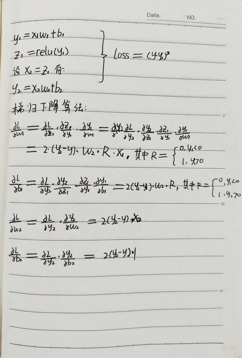
但这样实现的神经网络准确率很低,大概在40%左右,我猜测可能是激活函数和损失函数选取不太好的原因,于是乎重写了一份全连接神经网络的代码:
第二个(代码未被注释的部分),是基于交叉熵实现的损失函数,三层神经网络结构,采用了one_hot编码,隐藏层使用的relu激活函数,输出层使用的 softmax 激活函数,递归下降算法的实现以及求梯度的推导过程如下:
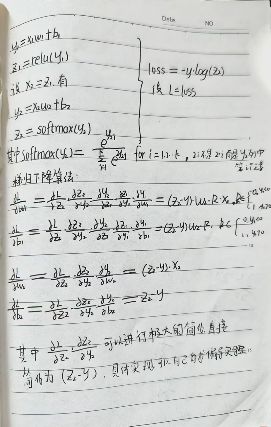
这次实现的全连接神经网络还可以,在使用不同参数的时候,准确率最低也有85%左右,最高能达到 96%上下。
代码实现
# import io
# from struct import pack,unpack
# import random
# from PIL import Image
# import numpy as np
# import matplotlib.pyplot as plt
# import time

# PIXEL = -1
# WIDTH = -1
# LENGTH = -1
# def set_randon_seed(seed):
#     random.seed(seed)

# def read_pic(pic_num,label_path = "./mnist/train-labels.idx1-ubyte",images_path = "./mnist/train-images.idx3-ubyte"):
#     global PIXEL,WIDTH,LENGTH
#     fp_label = open(label_path,'rb')
#     label_data = fp_label.read()
#     io_label = io.BytesIO(label_data)

#     fp_image = open(images_path,'rb')
#     image_data = fp_image.read()
#     io_image = io.BytesIO(image_data)

#     assert 0x00000801 == unpack(">I",io_label.read(4))[0]
#     assert 0x00000803 == unpack(">I",io_image.read(4))[0]
#     all_size = unpack(">I",io_label.read(4))[0]
#     io_image.read(4)
#     dx = unpack(">I",io_image.read(4))[0]
#     dy = unpack(">I",io_image.read(4))[0]
#     PIXEL = dx * dy
#     LENGTH = dx
#     WIDTH = dy


#     image_all = [io_image.read(PIXEL) for _ in range(all_size) ]
#     labels_all = [io_label.read(1) for _ in range(all_size)]
#     # random get pic
#     random_list = random.sample(range(all_size), pic_num)

#     image_list = []
#     labels_list = []
#     for i in random_list:
#         image_list.append( list(image_all[i]))
#         labels_list.append(labels_all[i][0])

#     return image_list,labels_list


# # 实际上,数据集提供的是二值图像,即灰白图片,0 代表白色,255 代表黑色,其他值介于0到255之间
# def pt_image(image_list):
#     image_np = np.array(image_list)
#     two_dim_array = image_np.reshape(-1, WIDTH)
#     image = Image.fromarray(two_dim_array.astype(np.uint8), mode='L')
#     image.show()

# def conver2one_hot(labels):
#     res=np.eye(10)[labels]
#     return res

# def fit(train_dataset,train_labels,lr,epochs,hidden_node):
#     train_dataset_np = np.array(train_dataset)
#     x = 2 * train_dataset_np / 255 -1        # 转化成浮点数张量
#     y = np.array(train_labels)
#     y = conver2one_hot(y)

#     w1 = np.random.randn(PIXEL,hidden_node)*np.sqrt(2. / PIXEL)         # 形成 PIXEL行,hidden_node列矩阵,大小取值为标准正态分布 / 20
#     b1 = np.zeros((1,hidden_node))
#     w2 = np.random.randn(hidden_node,10)*np.sqrt(2. / hidden_node)
#     b2 = np.zeros((1,10))
#     list_loss = np.zeros([epochs])  # ===》 初始化一个长度为 epochs 的数组,用于记录每一轮训练结束后的损失值。
#     list_epoch = np.arange(epochs)
#     for epoch in range(epochs):
#         y1 = x@w1 + b1                      #会自动广播的, np.broadcast_to(b1,x.shape(0),500)          # ===> 计算: x*w1 + b1
#         z1 = active_relu(y1)  # 通过激活函数                          # ===> 通过relu激活函数!
#         # 第二层计算 [b, 256] => [b, 128]
#         y2 = z1@w2 + b2

#         loss = np.square(y - y2)
#         loss = np.mean(loss)                             # 计算均方差
#         list_loss[epoch] = loss

#         # 下面求自动梯度
#         # 自动梯度,需要求梯度的张量有[w1,b1,w2,b2,w3,b3]
#         grads = get_gradient(loss, [w1,b1,w2,b2],[x,z1,y,y1,y2,z1])            # 返回一个包含每个变量梯度的列表
#         w1 -= lr * grads[0]                                # 实际上就是梯度公式:x_{n+1} = x_n - lr * 梯度
#         b1 -= lr * grads[1]                                #    即在不断的更新w、b中
#         w2 -= lr * grads[2]
#         b2 -= lr * grads[3]
#     return w1,b1,w2,b2


# start_ti = time.time()

# def active_relu(x): # 设置 relu激活函数
#     return np.where(x > 0, x, 0)

# def get_gradient(loss,wbs,vals):
#     w1 = wbs[0]
#     b1 = wbs[1]
#     w2 = wbs[2]
#     b2 = wbs[3]

#     x1 = vals[0]
#     x2 = vals[1]


#     y = vals[2]
#     y1 = vals[3]
#     y2 = vals[4]
#     z1 = vals[5]
#     m = y.shape[0]  # 样本数量
#     grads_w1 = (x1.T @ ((2*(y2-y)) @ w2.T * np.where(y1 < 0,0,1))) / m
#     grads_b1 = (np.sum((2*(y2-y)) @ w2.T * np.where(y1 < 0,0,1),axis=0,keepdims=True)) / m

#     grads_w2 = (x2.T @ (2*(y2-y) )) / m
#     grads_b2 = np.sum(2*(y2-y),axis=0,keepdims=True) / m

#     return [grads_w1,grads_b1,grads_w2,grads_b2]

# def predict(x_new,w1,b1,w2,b2):
#     y1 = x_new@w1 + b1                      #会自动广播的, np.broadcast_to(b1,x.shape(0),500)          # ===> 计算: x*w1 + b1
#     z1 = active_relu(y1)  # 通过激活函数                          # ===> 通过relu激活函数!
#     out = z1@w2 + b2
#     predictions = np.argmax(out,axis=1)

#     return predictions


# lr_list = [0.01,0.001,0.0001]
# for learing_rate in lr_list:
#     lr = learing_rate
#     epochs = 100
#     hidden_node = 1000
#     dataset_num = 20000
#     test_num = 200

#     set_randon_seed(0)
#     train_dataset,train_labels = read_pic(dataset_num)
#     test_dataset,test_labels = read_pic(test_num,label_path="./mnist/t10k-labels.idx1-ubyte",images_path="./mnist/t10k-images.idx3-ubyte")
#     w1, b1, w2, b2 = fit(train_dataset,train_labels,lr,epochs,hidden_node)
#     end_ti = time.time()
#     print(end_ti-start_ti)


#     st2 = time.time()

#     # 下面来预测图片:
#     correct_num = 0
#     for i in range(test_num):
#         new_image = test_dataset[i]  # 例如,使用验证集的第一张图像作为新图像
#         train_dataset_np = np.array(new_image)
#         x_new = 2 * train_dataset_np / 255 -1        # 转化成浮点数张量
#         predicted_num = predict(x_new, w1, b1, w2, b2)
#         if predicted_num == test_labels[i]:
#             correct_num += 1
#     print(f"when hidden node = {hidden_node} 、learning rate = {lr} , the accuracy_rate is {correct_num / test_num}")

#     end2 = time.time()
#     print(end2 - st2)


# # 34.15685439109802
# # when hidden node = 500 、learning rate = 0.1 , the accuracy_rate is 0.14
# # 0.04505658149719238
# # 72.59895038604736
# # when hidden node = 500 、learning rate = 0.01 , the accuracy_rate is 0.41
# # 0.04684591293334961
# # 110.56910133361816
# # when hidden node = 500 、learning rate = 0.001 , the accuracy_rate is 0.43
# # 0.04493856430053711
# # 148.3223340511322
# # when hidden node = 500 、learning rate = 0.0001 , the accuracy_rate is 0.14


import io
from struct import pack, unpack
import random
from PIL import Image
import numpy as np
import matplotlib.pyplot as plt
import time

PIXEL = -1
WIDTH = -1
LENGTH = -1  # 修正拼写错误

def set_random_seed(seed):
    random.seed(seed)
    np.random.seed(seed)  # 同时设置 NumPy 的随机种子

def read_pic(pic_num, label_path="./mnist/train-labels.idx1-ubyte", images_path="./mnist/train-images.idx3-ubyte"):
    global PIXEL, WIDTH, LENGTH
    with open(label_path, 'rb') as fp_label:
        label_data = fp_label.read()
    io_label = io.BytesIO(label_data)

    with open(images_path, 'rb') as fp_image:
        image_data = fp_image.read()
    io_image = io.BytesIO(image_data)

    assert 0x00000801 == unpack(">I", io_label.read(4))[0], "Label file magic number mismatch"
    assert 0x00000803 == unpack(">I", io_image.read(4))[0], "Image file magic number mismatch"
    all_size = unpack(">I", io_label.read(4))[0]
    io_image.read(4)  # Skip number of images again
    dx = unpack(">I", io_image.read(4))[0]
    dy = unpack(">I", io_image.read(4))[0]
    PIXEL = dx * dy
    LENGTH = dx
    WIDTH = dy

    image_all = [io_image.read(PIXEL) for _ in range(all_size)]
    labels_all = [io_label.read(1) for _ in range(all_size)]

    # 随机选择 pic_num 张图片
    random_list = random.sample(range(all_size), pic_num)

    image_list = []
    labels_list = []
    for i in random_list:
        image_list.append(list(image_all[i]))
        labels_list.append(labels_all[i][0])

    return image_list, labels_list

def pt_image(image_list):
    image_np = np.array(image_list)
    two_dim_array = image_np.reshape(-1, WIDTH)
    image = Image.fromarray(two_dim_array.astype(np.uint8), mode='L')
    image.show()

def conver2one_hot(labels):
    res = np.eye(10)[labels]
    return res

def active_relu(x):
    return np.maximum(0, x)

def softmax(x):
    # 为了数值稳定性,减去每行的最大值
    e_x = np.exp(x - np.max(x, axis=1, keepdims=True))
    return e_x / np.sum(e_x, axis=1, keepdims=True)

def fit(train_dataset, train_labels, lr, epochs, hidden_node):
    train_dataset_np = np.array(train_dataset)
    x = train_dataset_np / 255.0        # 归一化到 [0, 1]
    y = np.array(train_labels)
    y = conver2one_hot(y)  # one-hot 编码

    # 初始化权重和偏置
    w1 = np.random.randn(PIXEL, hidden_node) * np.sqrt(2. / PIXEL)      # He 初始化
    b1 = np.zeros((1, hidden_node))
    w2 = np.random.randn(hidden_node, 10) * np.sqrt(2. / hidden_node)   # He 初始化
    b2 = np.zeros((1, 10))
    list_loss = np.zeros([epochs])
    list_epoch = np.arange(epochs)

    for epoch in range(epochs):
        # 前向传播
        y1 = x @ w1 + b1
        z1 = active_relu(y1)
        y2 = z1 @ w2 + b2
        z2 = softmax(y2)

        # 计算交叉熵损失
        loss = -np.sum(y * np.log(z2 + 1e-8)) / y.shape[0]      # 1e-8 是为了 避免数值上的对数计算错误,具体来说,是为了防止对 零值 进行对数运算。
        list_loss[epoch] = loss

        # 反向传播
        delta2 = (z2 - y) / y.shape[0]  # 输出层梯度
        grads_w2 = z1.T @ delta2
        grads_b2 = np.sum(delta2, axis=0, keepdims=True)

        delta1 = (delta2 @ w2.T) * (y1 > 0)  # ReLU 导数
        grads_w1 = x.T @ delta1
        grads_b1 = np.sum(delta1, axis=0, keepdims=True)

        # 更新权重和偏置
        w1 -= lr * grads_w1
        b1 -= lr * grads_b1
        w2 -= lr * grads_w2
        b2 -= lr * grads_b2

        # 可选:打印损失
        if (epoch + 1) % 10 == 0 or epoch == 0:
            print(f"Epoch {epoch+1}/{epochs}, Loss: {loss:.4f}")

    # 绘制损失曲线
    # plt.plot(list_epoch, list_loss)
    # plt.xlabel('Epoch')
    # plt.ylabel('Loss')
    # plt.title('Training Loss over Epochs')
    # plt.show()

    return w1, b1, w2, b2

def predict(x_new, w1, b1, w2, b2):
    y1 = x_new @ w1 + b1
    z1 = active_relu(y1)
    y2 = z1 @ w2 + b2
    z2 = softmax(y2)
    predictions = np.argmax(z2, axis=1)  # 选择概率最大的类别
    return predictions  # 返回整个数组

# 测试学习率

# lr_list = [1,0.01, 0.001, 0.0001]
# for learning_rate in lr_list:
#     lr = learning_rate
#     epochs = 200
#     hidden_node = 500
#     dataset_num = 20000
#     test_num = 200

#     set_random_seed(0)
#     train_dataset, train_labels = read_pic(dataset_num)
#     test_dataset, test_labels = read_pic(test_num, label_path="./mnist/t10k-labels.idx1-ubyte", images_path="./mnist/t10k-images.idx3-ubyte")

#     train_start = time.time()
#     w1, b1, w2, b2 = fit(train_dataset, train_labels, lr, epochs, hidden_node)
#     train_end = time.time()
#     print(f"Training time: {train_end - train_start:.2f} seconds")

#     predict_start = time.time()

#     # 下面来预测图片:
#     x_test = np.array(test_dataset) / 255.0  # 归一化
#     y_test = np.array(test_labels)
#     y_pred = predict(x_test, w1, b1, w2, b2)
#     predict_end = time.time()

#     accuracy = np.mean(y_pred == y_test)
#     print(f"when hidden node = {hidden_node} 、learning rate = {lr} , the accuracy_rate is {accuracy:.4f}")

#     print(f"Prediction time: {predict_end - predict_start:.2f} seconds\n")


# 测试隐层节点
hidden_node_list = [500,1000,1500,2000]
for hidden_node_ in hidden_node_list:
    lr = 0.01
    epochs = 200
    hidden_node = hidden_node_
    dataset_num = 20000
    test_num = 200

    set_random_seed(0)
    train_dataset, train_labels = read_pic(dataset_num)
    test_dataset, test_labels = read_pic(test_num, label_path="./mnist/t10k-labels.idx1-ubyte", images_path="./mnist/t10k-images.idx3-ubyte")

    train_start = time.time()
    w1, b1, w2, b2 = fit(train_dataset, train_labels, lr, epochs, hidden_node)
    train_end = time.time()
    print(f"Training time: {train_end - train_start:.2f} seconds")

    predict_start = time.time()

    # 下面来预测图片:
    x_test = np.array(test_dataset) / 255.0  # 归一化
    y_test = np.array(test_labels)
    y_pred = predict(x_test, w1, b1, w2, b2)
    predict_end = time.time()

    # 计算准确率
    accuracy = np.mean(y_pred == y_test)
    print(f"when hidden node = {hidden_node} 、learning rate = {lr} , the accuracy_rate is {accuracy:.4f}")

    end2 = time.time()
    print(f"Prediction time: {predict_end - predict_start:.2f} seconds\n")
参考
https://gsy00517.github.io/machine-learning20191101192042/
https://www.cnblogs.com/LXP-Never/p/9979207.html
https://www.bilibili.com/video/BV1sJ411P7kt/?vd_source=87f7ad8544d4c3ad070c5c2ff28b7698

 浙公网安备 33010602011771号