


跟着东京大学镰谷研究室学习GWAS分析及可视化 - 实践
跟着东京大学镰谷研究室学习GWAS分析及可视化
REF:https://cloufield.github.io/GWASTutorial/
这里将给大家呈现GWAS分析的一般流程:从数据下载,前期质控,主成分分析,plink2表型关联分析到GWAS的可视化
1. Pre-GWAS(前期准备)
1.1 克隆相关文件
git clone https://github.com/Cloufield/GWASTutorial.git1.2 下载相关数据集
https://cloufield.github.io/GWASTutorial/01_Dataset/
cd GWASTutorial/01_Dataset
./download_sampledata.sh
# 1KG.EAS.auto.snp.norm.nodup.split.rare002.common015.missing.bed
# 1KG.EAS.auto.snp.norm.nodup.split.rare002.common015.missing.bim
# 1KG.EAS.auto.snp.norm.nodup.split.rare002.common015.missing.fam
Phenotype Simulation
表型模拟
Phenotypes were simply simulated using GCTA with the 1KG EAS dataset.
使用 GCTA 和 1KG EAS 数据集简单地模拟表型。
# 下载安装acta
wget https://yanglab.westlake.edu.cn/software/gcta/bin/gcta_1.94.0beta.zip
unzip gcta_1.94.0beta.zip
ln -s gcta_1.94.0beta/gcta64 /usr/local/bin/gcta
# 运行 GCTA
# 使用了GCTA软件的数据模拟功能,具体来说是在模拟一个病例对照研(Case-Control Study)的GWAS数据
gcta \
--bfile 1KG.EAS.auto.snp.norm.nodup.split.rare002.common015.missing \
--simu-cc 250 254 \ # 250个病例(cases),254个对照(controls)
--simu-causal-loci causal.snplist \ # 指定因果SNP的列表文件
--simu-hsq 0.8 \ # 遗传力为0.8,即80%的表型变异由遗传因素解释
--simu-k 0.5 \ # 疾病流行率为50%
--simu-rep 1 \ # 只进行1次重复模拟
--out 1kgeas_binary
# 1kgeas_binary.log
# 1kgeas_binary.par
# 1kgeas_binary.phen1.3 熟悉各种数据格式及其互相转换
https://cloufield.github.io/GWASTutorial/03_Data_formats/
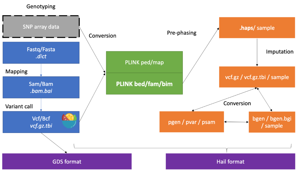
2. Genotype Data QC 基因型数据质量控制
https://cloufield.github.io/GWASTutorial/04_Data_QC/
# 打开官网https://www.cog-genomics.org/plink/1.9/
# 安装plink2
wget https://s3.amazonaws.com/plink2-assets/plink2_linux_x86_64_20251019.zip
unzip plink2_linux_x86_64_20251019.zip
# 安装plink1
wget https://s3.amazonaws.com/plink1-assets/plink_linux_x86_64_20250819.zip
unzip plink_linux_x86_64_20250819.zip
The functions we will learn in this tutorial:
我们将在本教程中学习的功能:
Calculating missing rate (call rate)
计算缺失率(呼叫率)
Calculating allele Frequency
计算等位基因频率
Conducting Hardy-Weinberg equilibrium exact test
进行 Hardy-Weinberg 平衡精确检验
Applying filters 应用过滤器
Conducting LD-Pruning
进行LD修剪
Calculating inbreeding F coefficient
计算近亲繁殖 F 系数
Conducting sample & SNP filtering (extract/exclude/keep/remove)
进行样品和 SNP 过滤(提取/排除/保留/去除)
Estimating IBD / PI_HAT
估计 IBD / PI_HAT
Calculating LD 计算 LD
Data management (make-bed/recode)
数据管理(补床/重新编码)
执行以下代码完成QC来获得干净的数据集
```bash
#!/bin/bash
#$ -S /bin/bash
export OMP_NUM_THREADS=4
genotypeFile="../01_Dataset/1KG.EAS.auto.snp.norm.nodup.split.rare002.common015.missing"
plink \
--bfile ${genotypeFile} \
--missing \ # 计算缺失率
--freq \ # 使用 PLINK1.9 计算变体的 MAF
--hardy \ # 使用 PLINK 计算 Hardy-Weinberg 平衡精确检验统计量
--out plink_results
plink2 \
--bfile ${genotypeFile} \
--freq \ # 使用 PLINK2 计算变异的替代等位基因频率
--out plink_results
plink \
--bfile ${genotypeFile} \
--maf 0.01 \ # 不含 MAF<0.01 的 SNP
--geno 0.01 \ # 过滤掉所有缺失率超过 0.02 的变体
--mind 0.02 \ # 过滤掉所有缺失率超过 0.02 的样本
--hwe 1e-6 \ # 过滤掉 Hardy-Weinberg 平衡精确检验 p 值低于所提供阈值的所有变体
--indep-pairwise 50 5 0.2 \ # 一个50个SNP的窗口,计算窗口中每对 SNP 之间的 LD,如果 LD 大于 0.2,则删除一对 SNP 中的一个;将窗口 5个 SNP 向前移动并重复该过程
--out plink_results
# Sample & SNP filtering (extract/exclude/keep/remove)
# 样品和 SNP 过滤(提取/排除/保留/去除)
plink \
--bfile ${genotypeFile} \
--extract plink_results.prune.in \ # 只使用通过LD筛选的独立SNP集合
--het \ # 计算每个样本的杂合度统计量
--out plink_results
# 使用 awk 创建具有极值 F 的个体样本列表
awk 'NR>1 && $6>0.1 || $6<-0.1 {print $1,$2}' plink_results.het > high_het.sample
plink \
--bfile ${genotypeFile} \
--extract plink_results.prune.in \
--genome \ # 执行核心计算。它会计算样本两两之间的IBS(状态同源)和IBD(血缘同源)统计量
--out plink_results
plink \
--bfile ${genotypeFile} \
--chr 22 \
--r2 \ # LD计算
--out plink_results
# 应用所有过滤器以获得干净的数据集
plink \
--bfile ${genotypeFile} \ # 指定输入的二进制基因型文件(前缀为 $genotypeFile的 .bed, .bim, .fam文件)
--geno 0.02 \ # SNP缺失率过滤:剔除在所有样本中缺失率高于2%的SNP位点
--mind 0.02 \ # 样本缺失率过滤:剔除基因型缺失率高于2%的样本
--hwe 1e-6 \ # 哈迪-温伯格平衡过滤:剔除显著偏离哈迪-温伯格平衡的SNP(p值 < 1e-6),这通常是基因分型错误的指标
--remove high_het.sample \ # 移除异常样本:根据文件 high_het.sample中的列表移除杂合度异常的样本(这些样本可能受污染或存在近亲繁殖)
--keep-allele-order \ # 保持等位基因顺序:防止PLINK自动重新排列等位基因,确保REF和ALT等位基因的顺序与原始文件一致,这对于后续分析整合至关重要
--make-bed \ # 生成二进制文件:将质控后的数据输出为新的二进制格式文件(.bed, .bim, .fam),便于后续分析
--out sample_data.clean # 输出前缀3. 主成分分析 (PCA)
https://cloufield.github.io/GWASTutorial/05_PCA/
#!/bin/bash
plinkFile="../04_Data_QC/sample_data.clean"
outPrefix="plink_results"
threadnum=2
# 1. 准备阶段:排除高LD区域
plink \
--bfile ${plinkFile} \
--make-set high-ld-hg19.txt \ # 创建一个高LD区域SNP列表,排除那些已知的、LD结构异常复杂的基因组区域(如人类白细胞抗原HLA区域)
--write-set \
--out hild
# 2. LD剪枝:获取独立SNP集合
# pruning
plink2 \
--bfile ${plinkFile} \
--maf 0.01 \
--exclude hild.set \
--threads ${threadnum} \
--indep-pairwise 500 50 0.2 \
--out ${outPrefix}
# 3. 移除高亲缘关系样本
# remove related samples using knig-cuttoff
plink2 \
--bfile ${plinkFile} \
--extract ${outPrefix}.prune.in \
--king-cutoff 0.0884 \
--threads ${threadnum} \
--out ${outPrefix}
# 4. 主成分计算与投影
# 计算PCA
# pca after pruning and removing related samples
plink2 \
--bfile ${plinkFile} \
--keep ${outPrefix}.king.cutoff.in.id \
--extract ${outPrefix}.prune.in \
--freq counts \
--threads ${threadnum} \
--pca approx allele-wts \
--out ${outPrefix}
# 投影到所有样本
# projection (related and unrelated samples)
plink2 \
--bfile ${plinkFile} \
--threads ${threadnum} \
--read-freq ${outPrefix}.acount \
--score ${outPrefix}.eigenvec.allele 2 6 header-read no-mean-imputation variance-standardize \
--score-col-nums 7-16 \
--out ${outPrefix}_projected
# ${outPrefix}.eigenval:记录每个主成分所解释的方差大小。
# ${outPrefix}.eigenvec:记录每个样本在前几个主成分上的得分(坐标)。这个文件通常用于绘制PCA散点图,直观展示样本的群体结构。
# ${outPrefix}_projected.sscore:所有样本的投影后主成分得分文件。这个文件就是后续GWAS分析中需要作为协变量输入的文件。- 理解PCA在GWAS中的作用
- 在GWAS中,群体结构 是导致假阳性关联的主要原因之一。例如,如果某个SNP在病例组中频率高是因为该SNP在某个祖先成分占比较高的亚群中本身频率就高,而该亚群恰好因其他因素(如环境、文化)有更高的患病率,就会产生虚假关联。PCA产生的主成分可以有效量化样本的祖先背景差异。在后续进行基因型-表型关联分析时(例如使用逻辑回归或混合线性模型),将前几个主成分作为协变量纳入模型,可以校正掉这些祖先差异造成的虚假关联,大大提升结果的可靠性
3.1 绘制PCA图
import pandas as pd
import matplotlib.pyplot as plt
import seaborn as sns
plt.style.use('default')
# 导入数据
pca = pd.read_table("/mnt/d/01_study/04_GWAS教程/GWASTutorial/05_PCA/plink_results_projected.sscore",sep="\t")
print(pca.shape)
pca.head()(500, 14)| #FID | IID | ALLELE_CT | NAMED_ALLELE_DOSAGE_SUM | PC1_AVG | PC2_AVG | PC3_AVG | PC4_AVG | PC5_AVG | PC6_AVG | PC7_AVG | PC8_AVG | PC9_AVG | PC10_AVG | |
|---|---|---|---|---|---|---|---|---|---|---|---|---|---|---|
| 0 | HG00403 | HG00403 | 390256 | 390256 | -0.002903 | 0.024865 | -0.010041 | -0.009576 | 0.006942 | 0.002221 | -0.008219 | -0.001130 | 0.003352 | -0.004364 |
| 1 | HG00404 | HG00404 | 390696 | 390696 | 0.000141 | 0.027965 | -0.025389 | 0.005825 | -0.002747 | -0.006574 | -0.011372 | 0.007771 | 0.015978 | -0.017931 |
| 2 | HG00406 | HG00406 | 388524 | 388524 | -0.007074 | 0.031545 | 0.004370 | 0.001262 | -0.011491 | 0.005403 | 0.006177 | 0.004497 | -0.000846 | 0.002172 |
| 3 | HG00407 | HG00407 | 388808 | 388808 | -0.006840 | 0.025073 | 0.006527 | -0.006797 | -0.011605 | 0.010242 | -0.013987 | 0.006177 | 0.013896 | -0.008327 |
| 4 | HG00409 | HG00409 | 391646 | 391646 | -0.000399 | 0.029033 | 0.018935 | 0.001360 | 0.029043 | -0.009415 | 0.017134 | -0.013041 | 0.025343 | -0.023163 |
ped = pd.read_table("/mnt/d/01_study/04_GWAS教程/GWASTutorial/01_Dataset/integrated_call_samples_v3.20130502.ALL.panel",sep="\t")
print(pca.shape)
ped.head()
(500, 14)| sample | pop | super_pop | gender | Unnamed: 4 | Unnamed: 5 | |
|---|---|---|---|---|---|---|
| 0 | HG00096 | GBR | EUR | male | NaN | NaN |
| 1 | HG00097 | GBR | EUR | female | NaN | NaN |
| 2 | HG00099 | GBR | EUR | female | NaN | NaN |
| 3 | HG00100 | GBR | EUR | female | NaN | NaN |
| 4 | HG00101 | GBR | EUR | male | NaN | NaN |
# 将PCA结果和人群信息进行合并
pcaped=pd.merge(pca,ped,right_on="sample",left_on="IID",how="inner")
print(pcaped.shape)
pcaped.head()
(500, 20)| #FID | IID | ALLELE_CT | NAMED_ALLELE_DOSAGE_SUM | PC1_AVG | PC2_AVG | PC3_AVG | PC4_AVG | PC5_AVG | PC6_AVG | PC7_AVG | PC8_AVG | PC9_AVG | PC10_AVG | sample | pop | super_pop | gender | Unnamed: 4 | Unnamed: 5 | |
|---|---|---|---|---|---|---|---|---|---|---|---|---|---|---|---|---|---|---|---|---|
| 0 | HG00403 | HG00403 | 390256 | 390256 | -0.002903 | 0.024865 | -0.010041 | -0.009576 | 0.006942 | 0.002221 | -0.008219 | -0.001130 | 0.003352 | -0.004364 | HG00403 | CHS | EAS | male | NaN | NaN |
| 1 | HG00404 | HG00404 | 390696 | 390696 | 0.000141 | 0.027965 | -0.025389 | 0.005825 | -0.002747 | -0.006574 | -0.011372 | 0.007771 | 0.015978 | -0.017931 | HG00404 | CHS | EAS | female | NaN | NaN |
| 2 | HG00406 | HG00406 | 388524 | 388524 | -0.007074 | 0.031545 | 0.004370 | 0.001262 | -0.011491 | 0.005403 | 0.006177 | 0.004497 | -0.000846 | 0.002172 | HG00406 | CHS | EAS | male | NaN | NaN |
| 3 | HG00407 | HG00407 | 388808 | 388808 | -0.006840 | 0.025073 | 0.006527 | -0.006797 | -0.011605 | 0.010242 | -0.013987 | 0.006177 | 0.013896 | -0.008327 | HG00407 | CHS | EAS | female | NaN | NaN |
| 4 | HG00409 | HG00409 | 391646 | 391646 | -0.000399 | 0.029033 | 0.018935 | 0.001360 | 0.029043 | -0.009415 | 0.017134 | -0.013041 | 0.025343 | -0.023163 | HG00409 | CHS | EAS | male | NaN | NaN |
# 绘制图像
plt.figure(figsize=(4,4))
sns.scatterplot(data=pcaped,x="PC1_AVG",y="PC2_AVG",hue="pop",s=50)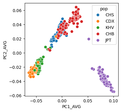
4. 对pre-GWAS data利用plink2进行GWAS分析
#!/bin/bash
export OMP_NUM_THREADS=1
genotypeFile="../04_Data_QC/sample_data.clean" # 经过质控的基因型数据
phenotypeFile="../01_Dataset/1kgeas_binary.txt" # 表型文件
covariateFile="../05_PCA/plink_results_projected.sscore" # 协变量文件(通常包含PCA结果)
covariateCols=6-10 # 指定使用协变量文件中的第6到10列(通常是前几个主成分)
colName="B1" # 指定要分析的表型在表型文件中的列名
threadnum=2
plink2 \
--bfile ${genotypeFile} \
--pheno ${phenotypeFile} \
--pheno-name ${colName} \
--maf 0.01 \ # 过滤掉次要等位基因频率低于0.01的罕见SNP
--covar ${covariateFile} \
--covar-col-nums ${covariateCols} \
--glm hide-covar firth firth-residualize single-prec-cc \ # 执行广义线性模型关联分析。
--threads ${threadnum} \
--out 1kgeas
# hide-covar: 在结果中不输出协变量自身的统计量,使结果文件更简洁。
# firth: 核心方法:使用Firth逻辑回归,这对于处理病例-对照不平衡或罕见变异非常有效,能减少假阳性。
# firth-residualize: 在Firth回归中对协变量进行残差化处理,可能提高数值稳定性。
# single-prec-cc: 为病例-对照分析使用单一精度计算,可能是在计算效率和精度间的一种权衡5. 利用gwaslab进行GWAS可视化
# 安装gwaslab
conda env create -n gwaslab -c conda-forge python=3.12
conda activate gwaslab
pip install gwaslab
import gwaslab as glsumstats = gl.Sumstats("/mnt/d/01_study/04_GWAS教程/GWASTutorial/06_Association_tests/1kgeas.B1.glm.firth",fmt="plink2")#2025/11/01 16:27:03 GWASLab v3.6.9 https://cloufield.github.io/gwaslab/
2025/11/01 16:27:03 (C) 2022-2025, Yunye He, Kamatani Lab, GPL-3.0 license, gwaslab@gmail.com
2025/11/01 16:27:03 Python version: 3.12.12 | packaged by conda-forge | (main, Oct 22 2025, 23:25:55) [GCC 14.3.0]
2025/11/01 16:27:03 Start to load format from formatbook....
2025/11/01 16:27:03 -plink2 format meta info:
2025/11/01 16:27:03 - format_name : PLINK2 .glm.firth, .glm.logistic,.glm.linear
2025/11/01 16:27:03 - format_source : https://www.cog-genomics.org/plink/2.0/formats
2025/11/01 16:27:03 - format_version : Alpha 3.3 final (3 Jun)
2025/11/01 16:27:03 - last_check_date : 20220806
2025/11/01 16:27:03 -plink2 to gwaslab format dictionary:
2025/11/01 16:27:03 - plink2 keys: ID,#CHROM,POS,REF,ALT,A1,OBS_CT,A1_FREQ,BETA,LOG(OR)_SE,SE,T_STAT,Z_STAT,P,LOG10_P,MACH_R2,OR
2025/11/01 16:27:03 - gwaslab values: SNPID,CHR,POS,REF,ALT,EA,N,EAF,BETA,SE,SE,T,Z,P,MLOG10P,INFO,OR
2025/11/01 16:27:04 Start to initialize gl.Sumstats from file :/mnt/d/01_study/04_GWAS教程/GWASTutorial/06_Association_tests/1kgeas.B1.glm.firth
2025/11/01 16:27:05 -Reading columns : OBS_CT,ALT,REF,#CHROM,POS,A1,LOG(OR)_SE,A1_FREQ,P,OR,ID,Z_STAT
2025/11/01 16:27:05 -Renaming columns to : N,ALT,REF,CHR,POS,EA,SE,EAF,P,OR,SNPID,Z
2025/11/01 16:27:05 -Current Dataframe shape : 1128732 x 12
2025/11/01 16:27:05 -Initiating a status column: STATUS ...
2025/11/01 16:27:05 #WARNING! Version of genomic coordinates is unknown...
2025/11/01 16:27:06 NEA not available: assigning REF to NEA...
2025/11/01 16:27:06 -EA,REF and ALT columns are available: assigning NEA...
2025/11/01 16:27:06 -For variants with EA == ALT : assigning REF to NEA ...
2025/11/01 16:27:06 -For variants with EA != ALT : assigning ALT to NEA ...
2025/11/01 16:27:06 Start to reorder the columns...v3.6.9
2025/11/01 16:27:06 -Current Dataframe shape : 1128732 x 14 ; Memory usage: 108.34 MB
2025/11/01 16:27:06 -Reordering columns to : SNPID,CHR,POS,EA,NEA,EAF,SE,Z,P,OR,N,STATUS,REF,ALT
2025/11/01 16:27:06 Finished reordering the columns.
2025/11/01 16:27:06 -Trying to convert datatype for CHR: string -> Int64...Int64
2025/11/01 16:27:06 -Column : SNPID CHR POS EA NEA EAF SE Z P OR N STATUS REF ALT
2025/11/01 16:27:06 -DType : object Int64 int64 category category float64 float64 float64 float64 float64 int64 category category category
2025/11/01 16:27:06 -Verified: T T T T T T T T T T T T T T
2025/11/01 16:27:06 -Current Dataframe memory usage: 109.42 MB
2025/11/01 16:27:06 Finished loading data successfully!
2025/11/01 16:27:06 Path component detected: ['140008085564128']
2025/11/01 16:27:06 Creating path: ./140008085564128sumstats.data| SNPID | CHR | POS | EA | NEA | EAF | SE | Z | P | OR | N | STATUS | REF | ALT | |
|---|---|---|---|---|---|---|---|---|---|---|---|---|---|---|
| 0 | 1:15774:G:A | 1 | 15774 | A | G | 0.028283 | 0.394259 | -0.743515 | 0.457170 | 0.745920 | 495 | 9999999 | G | A |
| 1 | 1:15777:A:G | 1 | 15777 | G | A | 0.073737 | 0.250121 | -0.698790 | 0.484683 | 0.839640 | 495 | 9999999 | A | G |
| 2 | 1:57292:C:T | 1 | 57292 | T | C | 0.104675 | 0.215278 | 0.447106 | 0.654799 | 1.101040 | 492 | 9999999 | C | T |
| 3 | 1:77874:G:A | 1 | 77874 | A | G | 0.019153 | 0.462750 | 0.249285 | 0.803140 | 1.122270 | 496 | 9999999 | G | A |
| 4 | 1:87360:C:T | 1 | 87360 | T | C | 0.023139 | 0.439532 | 1.171570 | 0.241371 | 1.673540 | 497 | 9999999 | C | T |
| ... | ... | ... | ... | ... | ... | ... | ... | ... | ... | ... | ... | ... | ... | ... |
| 1128727 | 22:51217954:G:A | 22 | 51217954 | A | G | 0.033199 | 0.362168 | -0.995476 | 0.319505 | 0.697307 | 497 | 9999999 | G | A |
| 1128728 | 22:51218377:G:C | 22 | 51218377 | C | G | 0.033333 | 0.362212 | -0.994434 | 0.320012 | 0.697539 | 495 | 9999999 | G | C |
| 1128729 | 22:51218615:T:A | 22 | 51218615 | A | T | 0.033266 | 0.362476 | -1.029200 | 0.303385 | 0.688624 | 496 | 9999999 | T | A |
| 1128730 | 22:51222100:G:T | 22 | 51222100 | T | G | 0.039157 | 0.323177 | 0.617831 | 0.536687 | 1.221000 | 498 | 9999999 | G | T |
| 1128731 | 22:51239678:G:T | 22 | 51239678 | T | G | 0.034137 | 0.354398 | 0.578612 | 0.562851 | 1.227600 | 498 | 9999999 | G | T |
1128732 rows × 14 columns
sumstats.get_lead(sig_level=5e-8)2025/11/01 16:28:49 Start to extract lead variants...v3.6.9
2025/11/01 16:28:49 -Current Dataframe shape : 1128732 x 14 ; Memory usage: 109.42 MB
2025/11/01 16:28:49 -Processing 1128732 variants...
2025/11/01 16:28:49 -Significance threshold : 5e-08
2025/11/01 16:28:49 -Sliding window size: 500 kb
2025/11/01 16:28:49 -Using P for extracting lead variants...
2025/11/01 16:28:49 -Found 63 significant variants in total...
2025/11/01 16:28:49 -Identified 4 lead variants!
2025/11/01 16:28:49 Finished extracting lead variants.| SNPID | CHR | POS | EA | NEA | EAF | SE | Z | P | OR | N | STATUS | REF | ALT | |
|---|---|---|---|---|---|---|---|---|---|---|---|---|---|---|
| 54904 | 1:167562605:G:A | 1 | 167562605 | A | G | 0.391481 | 0.159645 | 7.69464 | 1.418880e-14 | 3.415790 | 493 | 9999999 | G | A |
| 113200 | 2:55587876:T:C | 2 | 55587876 | C | T | 0.313883 | 0.167300 | -8.02894 | 9.831720e-16 | 0.260998 | 497 | 9999999 | T | C |
| 549705 | 7:134326056:G:T | 7 | 134326056 | T | G | 0.134809 | 0.232018 | 7.10413 | 1.210840e-12 | 5.198050 | 497 | 9999999 | G | T |
| 1088750 | 20:42758834:T:C | 20 | 42758834 | T | C | 0.227273 | 0.184323 | -7.76905 | 7.907810e-15 | 0.238828 | 495 | 9999999 | T | C |
sumstats.plot_mqq(skip=2,anno=True)2025/11/01 16:29:19 Start to create MQQ plot...v3.6.9:
2025/11/01 16:29:19 -Genomic coordinates version: 99...
2025/11/01 16:29:19 #WARNING! Genomic coordinates version is unknown.
2025/11/01 16:29:19 -Genome-wide significance level to plot is set to 5e-08 ...
2025/11/01 16:29:19 -Raw input contains 1128732 variants...
2025/11/01 16:29:19 -MQQ plot layout mode is : mqq
2025/11/01 16:29:19 Finished loading specified columns from the sumstats.
2025/11/01 16:29:19 Start data conversion and sanity check:
2025/11/01 16:29:20 -Removed 0 variants with nan in CHR or POS column ...
2025/11/01 16:29:20 -Removed 0 variants with CHR <=0...
2025/11/01 16:29:20 -Removed 0 variants with nan in P column ...
2025/11/01 16:29:20 -Sanity check after conversion: 0 variants with P value outside of (0,1] will be removed...
2025/11/01 16:29:20 -Sumstats P values are being converted to -log10(P)...
2025/11/01 16:29:20 -Sanity check: 0 na/inf/-inf variants will be removed...
2025/11/01 16:29:20 -Converting data above cut line...
2025/11/01 16:29:20 -Maximum -log10(P) value is 15.007370498326086 .
2025/11/01 16:29:20 Finished data conversion and sanity check.
2025/11/01 16:29:20 Start to create MQQ plot with 8511 variants...
2025/11/01 16:29:20 -Creating background plot...
2025/11/01 16:29:20 Finished creating MQQ plot successfully!
2025/11/01 16:29:20 Start to extract variants for annotation...
2025/11/01 16:29:20 -Found 4 significant variants with a sliding window size of 500 kb...
2025/11/01 16:29:20 Finished extracting variants for annotation...
2025/11/01 16:29:20 Start to process figure arts.
2025/11/01 16:29:20 -Processing X ticks...
2025/11/01 16:29:20 -Processing X labels...
2025/11/01 16:29:20 -Processing Y labels...
2025/11/01 16:29:20 -Processing Y tick lables...
2025/11/01 16:29:20 -Processing Y labels...
2025/11/01 16:29:20 -Processing lines...
2025/11/01 16:29:20 Finished processing figure arts.
2025/11/01 16:29:20 Start to annotate variants...
2025/11/01 16:29:20 -Annotating using column CHR:POS...
2025/11/01 16:29:20 -Adjusting text positions with repel_force=0.03...
2025/11/01 16:29:20 Finished annotating variants.
2025/11/01 16:29:20 Start to create QQ plot with 8511 variants:
2025/11/01 16:29:20 -Plotting all variants...
2025/11/01 16:29:20 -Expected range of P: (0,1.0)
2025/11/01 16:29:20 -Lambda GC (MLOG10P mode) at 0.5 is 0.99002
2025/11/01 16:29:20 -Processing Y tick lables...
2025/11/01 16:29:20 Finished creating QQ plot successfully!
2025/11/01 16:29:20 Start to save figure...
2025/11/01 16:29:20 -Skip saving figure!
2025/11/01 16:29:20 Finished saving figure...
2025/11/01 16:29:20 Finished creating plot successfully!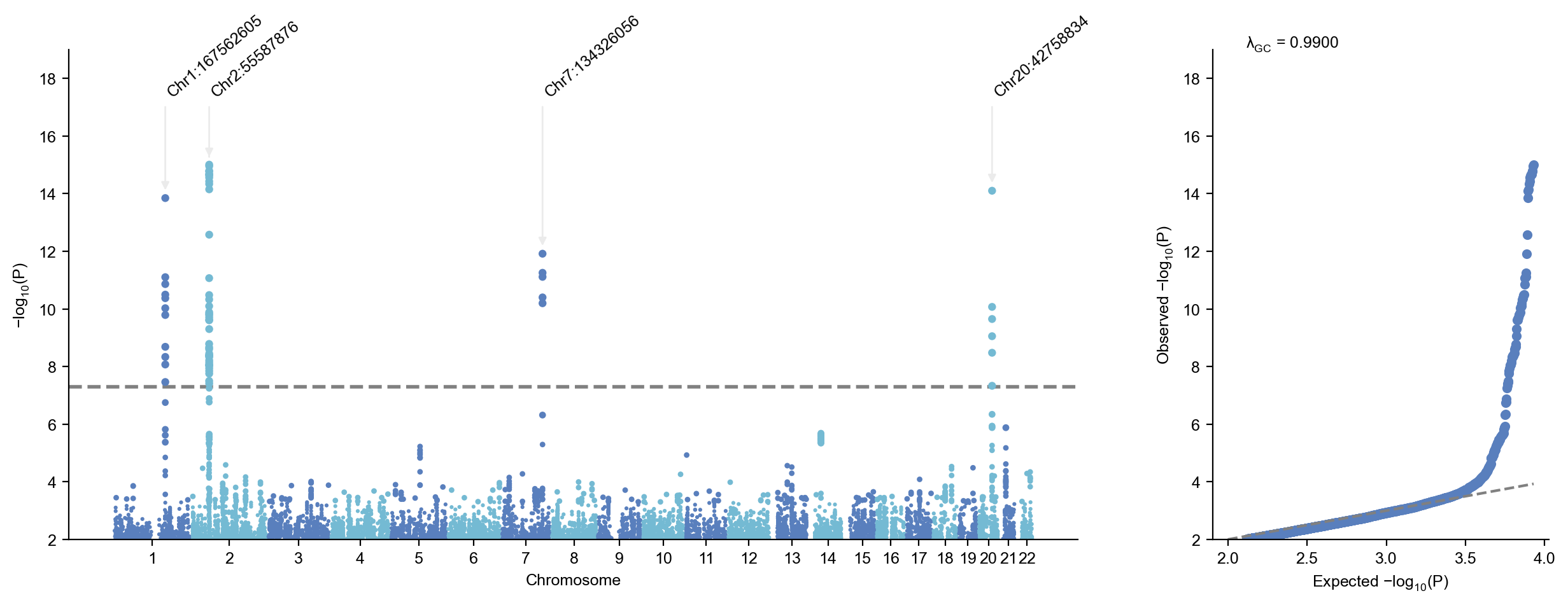

 浙公网安备 33010602011771号