GIS兼职日记-持续连载-至第83单

@ 20241112 & lth
开始时间：2025-08-07
更新时间：2025-11-19
PS：如果你也有相关的GIS数据处理、脚本模型开发定制化需求，欢迎联系我，微信:keylthing

比较简单的就不做详细说明了
1、SLDPRT转GEOJSON -- 20250807
2、MAPGIS转CAD -- 20250815
3、CAD图层的矢量数据空间校正-转GCJ02 -- 20250820
4、excel经纬度可视化为shp -- 20250821
5、mdb转cad -- 20250821
6、MAPGIS转shp -- 20250822
7、excel转shp -- 20250901
8、cad转shp -- 20250901
9、cad转shp -- 20250901
10、cad转shp -- 20250902
11、cad转shp -- 20250902
12、cad转shp -- 20250902
13、矢量融合拆分 -- 20250904
14、cad转shp -- 20250904
15、MAPGIS转shp -- 20250904
16、cad转shp -- 20250904
17、cad转shp -- 20250904
18、cad转shp -- 20250904
19、pdf矢量化 -- 20250904
20、shp转cad -- 20250905
21、stl转glb -- 20250908
22、kml转shp -- 20250908
23、双变量图 -- 20250909
24、监督分类 -- 20250910
25、林业图斑矢量绘制 -- 20250911
26、CAD笛子复刻 -- 20250912
27、3d柱状图 -- 20250915
28、重金属含量长江安徽段出图 -- 20250917
29、区位图 -- 20250917
30、民国二十年-长江淮河降雨推移图 -- 20250918
31、应急地图 -- 20250919
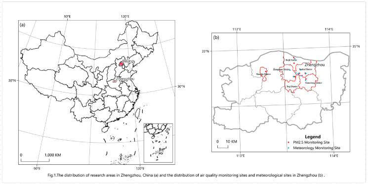
32、郑州监测点 -- 20250921
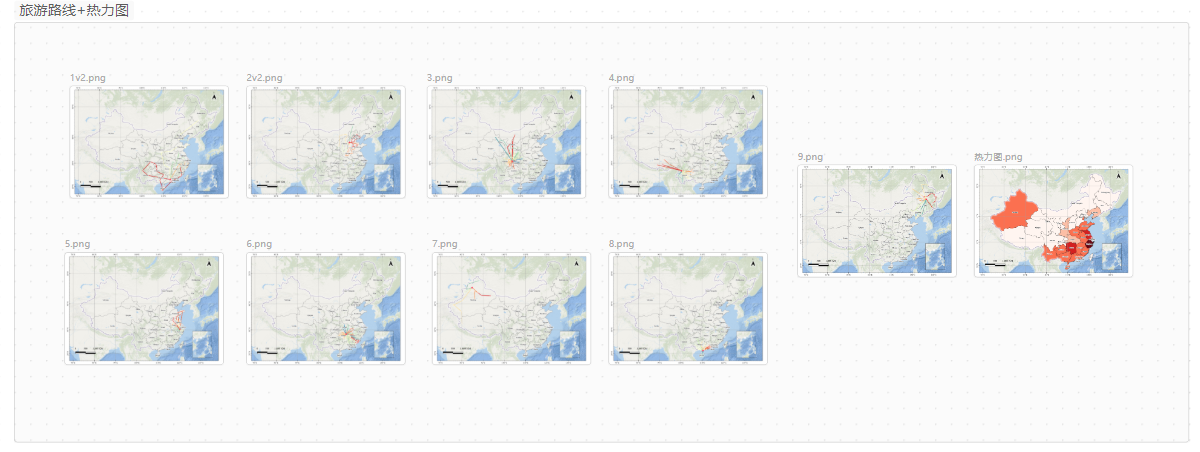
33、旅游线路+热力图 -- 20250925
34、栅格补值 -- 20250926
35、鸟类观赏路线绘制 -- 20250926
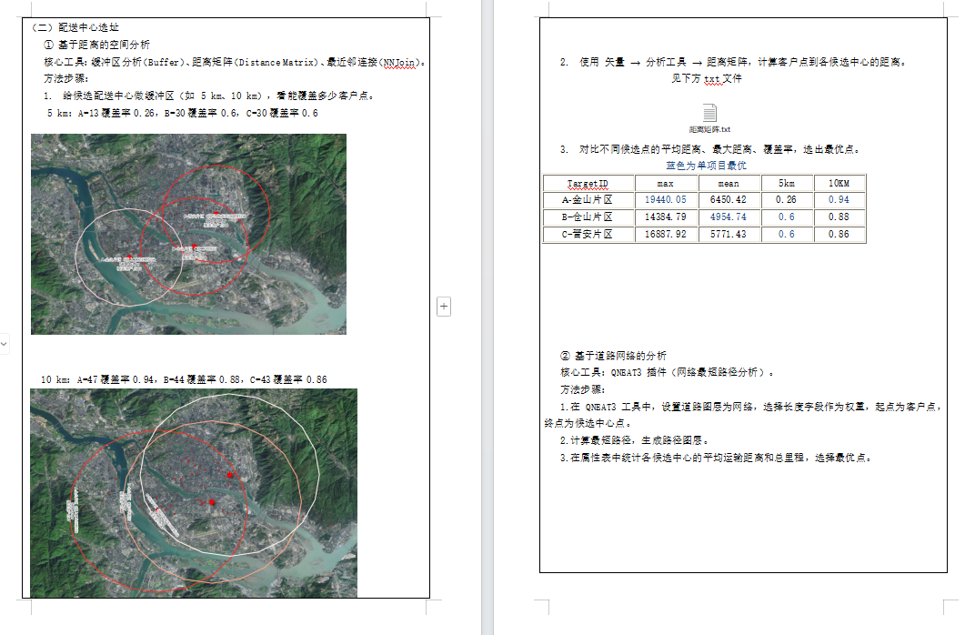
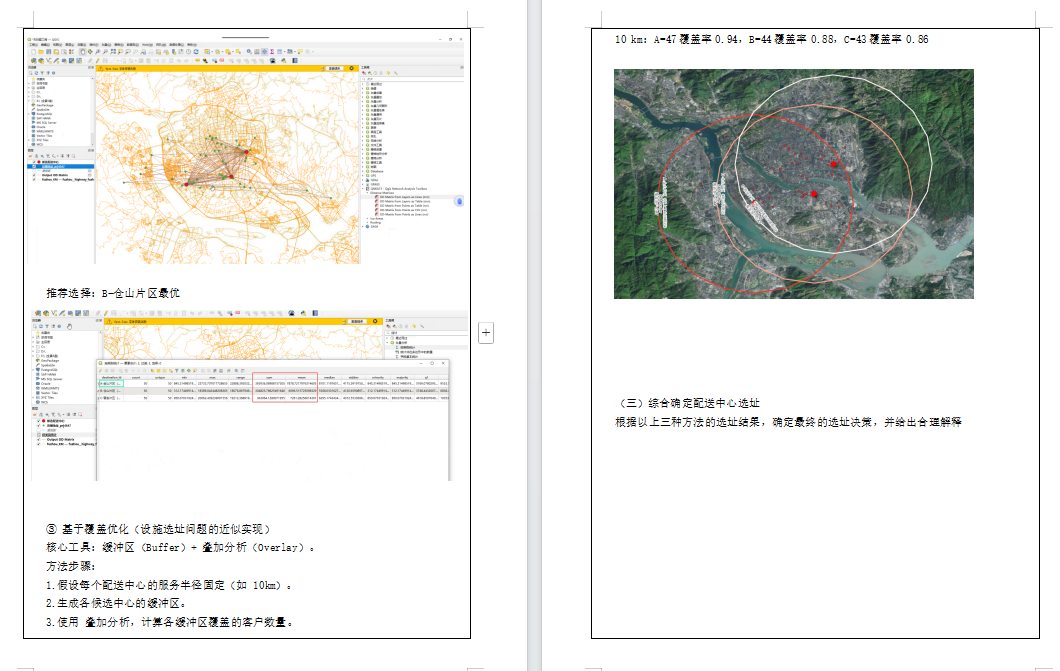
36、选址分析 -- 20250927
37、FOS滑坡失效概率计算 -- 20250927
38、混淆矩阵 -- 20251001
.........
68、postgre&qgis出图 -- 20251104
69、mysql&python出图 -- 20251104
70、GIS and Empirical Reasoning -- 20251112
83、GGRA30_Assign5_IntroArcGISOnline -- 20251119

1-SLDPRT转GEOJSON

客户需求和拆解

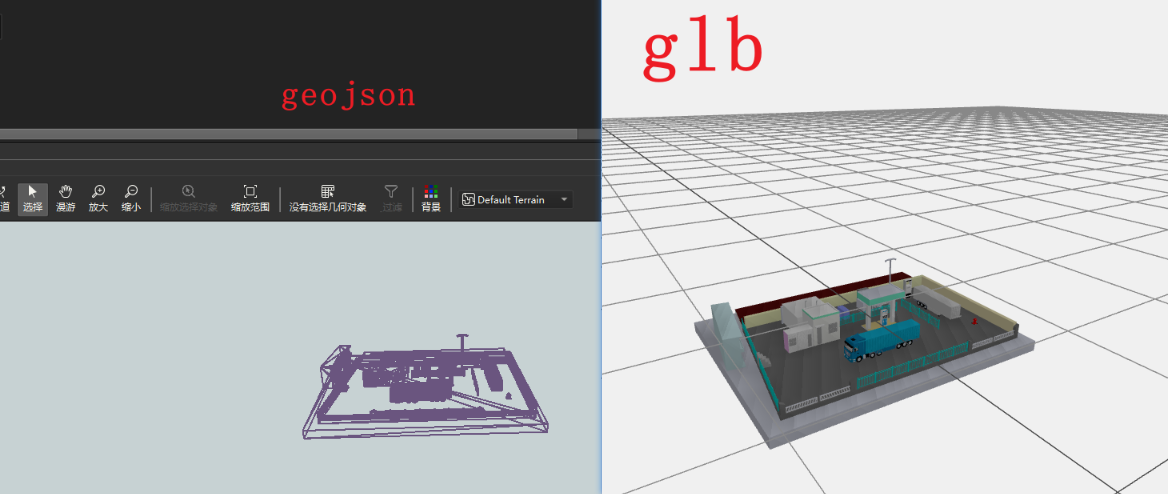
SLDPRT转GEOJSON想在web展示，那么我们主要是推荐他转成glb用在three.js中可视化
对于这个SLDPRT格式，我也是第一次接触，那么就用搜索大法了解一下，得知SLDPRT是SolidWorks这个软件的一个私有格式，主要是做一些3d模型的设计。
经过查询得知，一般都是推下载SolidWorks这个软件来进行格式转换，但是看到25G的软件大小，决定再查找一番。
果然，经过查询，发现了Crossmanager 2024 64 bit这款软件包含了大量3d类的数据转换

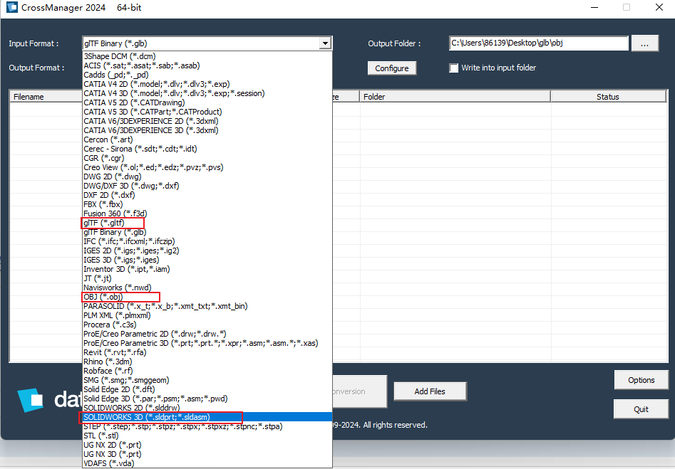
解决方案

那么再梳理一下客户需求，SLDPRT转GEOJSON显然是没法直接转换，那么我们一步步来拆解，首先我们可以用Crossmanager将SLDPRT转到obj，然后用fme读取obj转到geojosn

成果展示

2-MAPGIS转CAD

客户需求和拆解

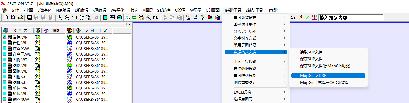
mapgis也是业内比较出名的国产软件，奈何之前没有接触过，也是花了40分钟才搞定这个简单需求
一样的先搜索有没有前人写好的开源软件，发现没有，最后通过询问群友和微信公众号得知需要下载mapgis和一个section的插件用来做转换（感谢群友）

解决方案

就很清晰了下载mapgis然后安装插件section，直接用mapgis将.MPJ这个我理解是工程文件打开，然后使用插件进行转换，生成后的dxf会自动保存到MPJ所在目录下
需要注意的是，如果不需要某个图层可以将其关闭，用cad或看图软件打开输出的dxf后，如果没有看到图形，双击鼠标滚轮做一个复位操作即可

成果展示

3-CAD图层的矢量数据空间校正-转GCJ02

客户需求和拆解

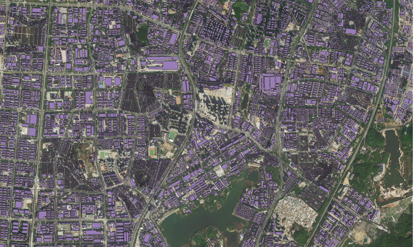
首先简单说一下需求，客户有个CAD矢量数据，他自己已经转成了shp，想把这几个图层校正到高德影像上实现重叠，那么这个也比较简单，但是也踩了一个坑后面细说

解决方案

我首先的思路就是，纯手工，我一般优先用qgis, 奈何发现qgis效率太慢，该换arcgispro效率起飞，
加载天地图做空间校正，矫正完之后再用qgis的插件做坐标转换为gcj02，最后叠加高德地图检查是否重叠
这里踩的坑是，其中一个矢量没有提前定义坐标系导致返工一次
这里写几个注意点：
1、CAD的图层转成shp一定要提前定义一下坐标系，如果他本来就没有，直接定义3857方便操作；
2、空间校正CAD的时候可以先用相似转换，把图层校正到大概位置，然后再用仿射进行精细化调优。

成果展示

4-excel经纬度可视化为shp

注意事项

这个比较简单就不赘述了，注意事项是excel的编码

5-mdb转cad

注意事项

这个比较简单就不赘述了，注意事项是一般cad需要计算面积长度什么的，所以最好转成投影坐标系

8-cad转shp

客户需求和拆解

autocad_entity、autocad_alyer、autocad_layer_color、autocad_layer_desc、aotocad_layer_frozen、autocad_layer_hidden、fme_text_size、fme_text_string、fme_type

9-cad转shp

注意事项

国内cad一般是投影坐标系：
1、x和y都是6同样位数基本是独立坐标系需要3/7参数进行校正；
3、x7/y8则是加上带号的，y的前两位数就是带号，带号通过带号计算中央子午线来确定3度带还是的6度带
4、x6/y7则是要么提前知道地区或给了中央子午线等，不然就只能一个个去套
5、1比1万基本要用3度带

20-shp转cad

注意事项

需要注意的是用FME写出cad的时候要选一下坐标系存储到哪里

21-stl转glb

注意事项

这个可以开个坑，一会补充细节

22-kml转shp

注意事项

目前我搜了一下没有现成的工具，要想将kml带属性转成shp,我这里工具选的是fme或python

用fme的话，关键点就是StringSearcher转换器，(?<=<td>).+?(?=</td>)，然后用AttributeExposer暴露出来把获取的字段

用python的话，关键点就是对description字段的处理
import xml.etree.ElementTree as ET
import os
from osgeo import ogr


def parse_kml_description(html_content):
    """
    解析 KML description 字段中的 HTML 表格，提取属性字典。
    
    参数:
        html_content (str): 描述字段的 HTML 内容（如 '<table>...</table>'）
    
    返回:
        dict: 提取的属性字典，例如 {'bh': '40339', 'name': '831774/2023', 'FID': '40338'}
    """
    # 尝试修复不完整的 HTML（比如缺少根标签）
    if not html_content.strip().startswith('<table'):
        # 查找第一个 <table> 开始位置
        start = html_content.find('<table')
        end = html_content.find('</table>')
        if start == -1 or end == -1:
            return {}
        html_content = html_content[start:end + 8]  # 截取完整 table

    try:
        # 使用 XML 解析器解析 HTML 表格
        root = ET.fromstring(html_content)
        
        # 如果根节点不是 <table>，尝试找子节点中的 <table>
        if root.tag != 'table':
            table = root.find('.//table')
            if table is not None:
                root = table
            else:
                return {}

        attr_dict = {}
        # 遍历所有表格行
        for row in root.findall('.//tr'):
            ths = row.findall('th')
            tds = row.findall('td')
            if len(ths) > 0 and len(tds) > 0:
                key = ths[0].text
                value = tds[0].text
                if key:  # 确保字段名不为空
                    attr_dict[key.strip()] = value.strip() if value else ''
        return attr_dict
    except ET.ParseError as e:
        print(f"HTML 解析失败: {e}")
        return {}


def convert_kml_to_shp(in_file, out_file):
    """
    将 KML 文件转换为 Shapefile，并从 description 中提取嵌套属性。

    参数:
        in_file (str): 输入 KML 文件路径。
        out_file (str): 输出 SHP 文件路径。
    """
    # 打开输入 KML 文件
    ds_in = ogr.Open(in_file)
    if ds_in is None:
        print(f"无法打开输入文件：{in_file}")
        return

    layer = ds_in.GetLayer(0)
    srs = layer.GetSpatialRef()  # 获取空间参考

    # 创建输出 Shapefile
    driver = ogr.GetDriverByName('ESRI Shapefile')
    # 删除已存在的输出文件（OGR 不会自动覆盖）
    if os.path.exists(out_file):
        driver.DeleteDataSource(out_file)
    ds_out = driver.CreateDataSource(out_file)
    if ds_out is None:
        print(f"无法创建输出文件：{out_file}")
        return

    # 获取输入图层定义
    layer_defn = layer.GetLayerDefn()
    geom_type = layer_defn.GetGeomType()

    # 创建输出图层（暂时无字段，后面动态添加）
    layer_out = ds_out.CreateLayer('output', srs=srs, geom_type=geom_type)

    # 存储已创建的字段名，避免重复创建
    created_fields = set()

    # === 第一步：遍历所有要素，提取 description 中的所有唯一字段名 ===
    print("正在扫描所有要素以提取字段...")
    all_attributes = set()
    features_data = []  # 临时存储每个要素的 geometry 和属性字典

    for feat_in in layer:
        desc = feat_in.GetField('description')  # 获取 description 字段
        if desc is not None:
            attrs = parse_kml_description(desc)
            all_attributes.update(attrs.keys())
            features_data.append({
                'geometry': feat_in.GetGeometryRef().Clone(),
                'attributes': attrs
            })
        else:
            features_data.append({
                'geometry': feat_in.GetGeometryRef().Clone(),
                'attributes': {}
            })

    # === 第二步：根据提取出的所有字段，创建 Shapefile 的字段 ===
    print(f"发现以下属性字段: {sorted(all_attributes)}")
    for field_name in sorted(all_attributes):
        # 检查字段名是否合法（Shapefile 字段名不能太长，且只能用字母数字下划线）
        safe_name = field_name.strip()
        if not safe_name.isidentifier():
            safe_name = ''.join(c if c.isalnum() or c == '_' else '_' for c in safe_name)
        if len(safe_name) > 10:  # Shapefile 字段名最多 10 字符
            safe_name = safe_name[:10]
        # 避免重复
        if safe_name not in created_fields:
            field_defn = ogr.FieldDefn(safe_name, ogr.OFTString)
            field_defn.SetWidth(254)
            layer_out.CreateField(field_defn)
            created_fields.add(safe_name)

    # 获取输出图层的要素定义
    feat_defn = layer_out.GetLayerDefn()

    # === 第三步：写入所有要素 ===
    for data in features_data:
        feat_out = ogr.Feature(feat_defn)
        feat_out.SetGeometry(data['geometry'])

        # 填充从 description 中提取的属性
        for key, value in data['attributes'].items():
            safe_key = key.strip()
            if not safe_key.isidentifier():
                safe_key = ''.join(c if c.isalnum() or c == '_' else '_' for c in safe_key)
            if len(safe_key) > 10:
                safe_key = safe_key[:10]
            if safe_key in created_fields:
                feat_out.SetField(safe_key, value)

        layer_out.CreateFeature(feat_out)
        feat_out = None  # 释放内存

    # 清理
    ds_out = None
    ds_in = None
    print(f"✅ 转换完成！已将 {len(features_data)} 个要素写入 {out_file}")

插入一个打包的知识点用Nuitka比pyinstaller要好很多，生成的exe要小很多大概是5倍，然后要注意的是pyqt5不太兼容Nuitka

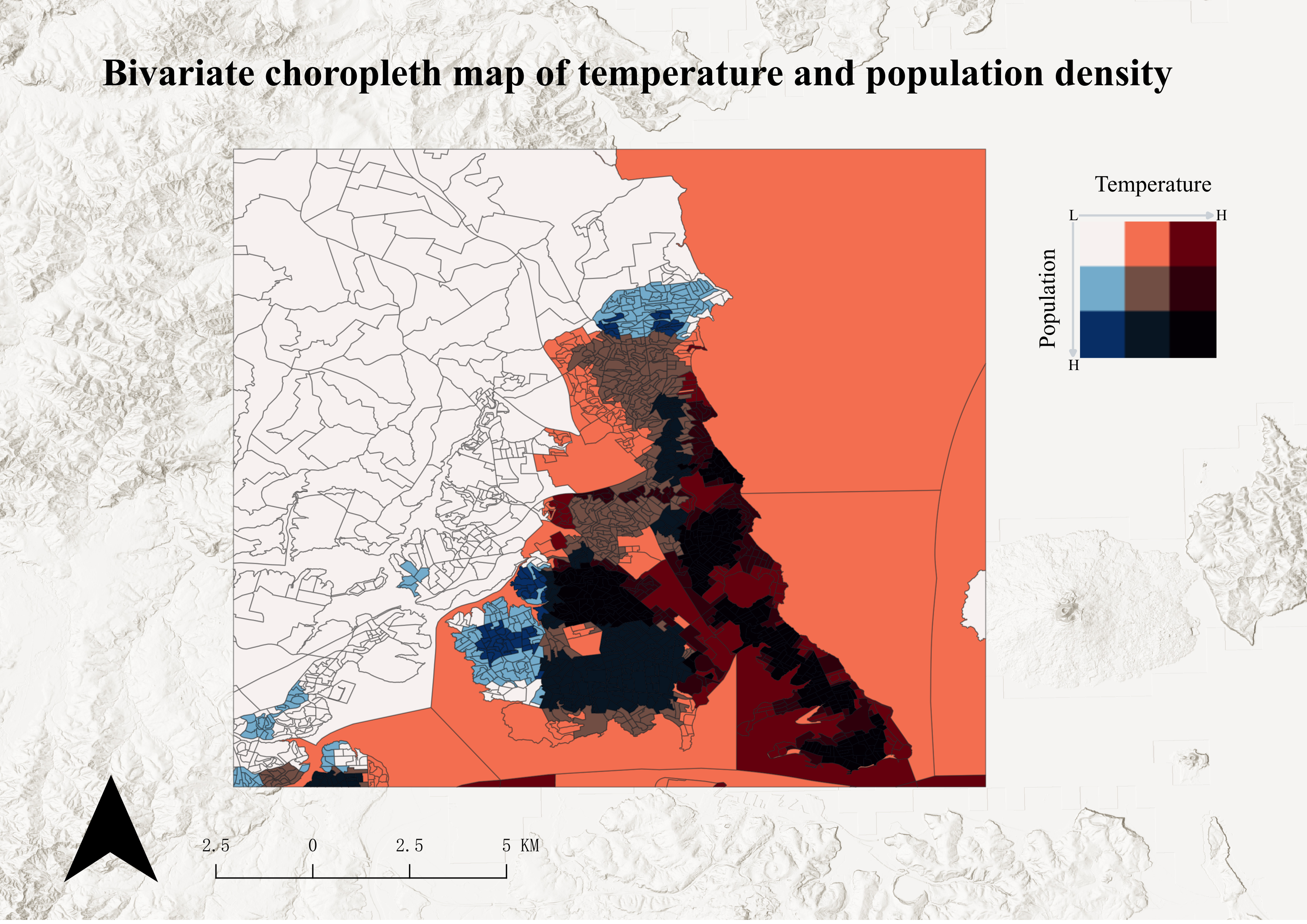
22-双变量图

注意事项

这个需求之前我也没有做过第一次弄，简单介绍一下就是一个研究区内，两个不同的要素属性，比如温度、人口两个字段, 直接对两个图层做渐变，一般是3个分级，上面的图层用正射叠加，然后关键点是做图例，用bivariate legend这个插件做图例，保存图片的时候用pdf这个格式，其他的没什么说的就是正常出图
数据这块：
人口https://landscan.ornl.gov/
温度https://climate.northwestknowledge.net/TERRACLIMATE/index_directDownloads.php

NC文件的处理

后面贴一个处理连续时间nc数据的求平均栅格的代码

import xarray as xr
import os
import numpy as np
import rioxarray # 用于地理空间处理和 GeoTIFF 导出
from typing import Optional

# 删除了对 osgeo.gdal 和 geopandas 的导入

# --- 辅助函数：交互式获取变量名 ---
def get_variable_choice(ds: xr.Dataset) -> Optional[str]:
    """
    打印数据集中的数据变量，并提示用户进行选择。
    """
    data_vars = list(ds.data_vars)
    if not data_vars:
        print("警告：NetCDF 文件中没有找到任何数据变量（Data Variables）。")
        return None

    print("-" * 50)
    print("文件中的 **可用数据变量** 及其描述如下：")
    for i, var in enumerate(data_vars):
        long_name = ds[var].attrs.get('long_name', '无描述信息')
        print(f"  [{i+1}] **{var}** (描述: {long_name})")
    print("-" * 50)
    
    while True:
        choice = input("请输入您要提取的**变量名**（例如：tmax）或对应的**数字序号**: ").strip()
        
        # 检查是否为数字序号
        if choice.isdigit():
            idx = int(choice) - 1
            if 0 <= idx < len(data_vars):
                return data_vars[idx]
        # 检查是否为变量名
        elif choice in data_vars:
            return choice
        
        print("输入无效。请确保输入正确的变量名或序号。")


# --- 1. 数据处理核心：读取并计算时间平均值 (强制设置 CRS) ---
def read_and_calculate_time_average(input_nc_file: str) -> Optional[xr.DataArray]:
    """
    读取 NetCDF 文件，交互式选择变量，计算时间平均值，并强制设置 WGS84 投影。
    """
    if not os.path.exists(input_nc_file):
        print(f"错误：输入 NC 文件未找到 -> {input_nc_file}")
        return None

    print(f"\n--- 1. 读取文件并计算平均值：{input_nc_file} ---")
    
    try:
        ds = xr.open_dataset(input_nc_file, chunks='auto')
        
        # 打印坐标信息
        print("  --- NetCDF 坐标信息 ---")
        print(ds.coords)
        print("  -------------------------")
        
        # 交互式选择变量
        chosen_var = get_variable_choice(ds)
        if chosen_var is None:
            return None

        da = ds[chosen_var]
        
        # 寻找时间维度
        time_dim = next((dim for dim in da.dims if dim.lower() in ['time', 't', 'times']), da.dims[0])
        print(f"  已选择变量：**{chosen_var}**")
        print(f"  识别到的时间维度为：'{time_dim}'")
        print(f"  正在计算时间维度上的平均值...")
        
        # 计算平均值
        mean_da = da.mean(dim=time_dim, skipna=True)
        
        # 关键步骤：强制设置 CRS 为 EPSG:4326 (WGS84)，解决 GeoTIFF 无投影问题
        if mean_da.rio.crs is None:
            mean_da = mean_da.rio.write_crs("EPSG:4326")
            print("  ✅ 已强制设置栅格 CRS 为 EPSG:4326 (WGS84)。")

        # 存储信息用于后续函数
        mean_da.attrs['original_variable_name'] = chosen_var
        
        return mean_da

    except Exception as e:
        print(f"错误：在读取或计算平均值过程中发生异常。详细错误信息：{e}")
        return None


# --- 2. 导出核心：设置地理信息并导出为 GeoTIFF ---
def export_to_geotiff(da: xr.DataArray, year: int, output_dir: str = '.'):
    """
    将 DataArray 导出为 GeoTIFF 文件，用于输出完整栅格。
    """
    chosen_var = da.attrs.get('original_variable_name', 'data')
    
    output_filename = f'{chosen_var}_average_{str(year)}.tif'
    output_path = os.path.join(output_dir, output_filename)
    
    # 确保输出目录存在
    os.makedirs(output_dir, exist_ok=True)
    
    print(f"\n--- 2. 导出 GeoTIFF：{output_path} ---")

    try:
        da.rio.to_raster(
            raster_path=output_path,
            dtype=np.float32, 
            compress='LZW'
        )
        
        print("\n" + "=" * 50)
        print(f"成功！GeoTIFF 文件已保存到 -> **{output_path}**")
        print("=" * 50)
        
    except Exception as e:
        print(f"错误：在保存 GeoTIFF 过程中发生异常。详细错误信息：{e}")
        if "[Errno 13]" in str(e):
             print("\n!!! 权限错误：请检查输出目录的写入权限或文件是否被占用。!!!")


# --- 3. 主流程函数 (简化版) ---
def main_process(
    input_nc_file: str, 
    year: int = 2023
):
    """
    串联读取、计算平均值和导出 GeoTIFF 的流程。
    """
    # 1. 计算时间平均值 (包含交互式变量选择和CRS设置)
    mean_da = read_and_calculate_time_average(input_nc_file)
    if mean_da is None:
        return

    # 获取脚本所在的目录作为输出目录
    output_dir = os.path.dirname(os.path.abspath(__file__)) if os.path.dirname(__file__) else '.'

    # 2. 导出完整的平均值栅格
    export_to_geotiff(mean_da, year, output_dir=output_dir)

    print("\n处理流程结束。")

# --- 调用主流程示例 ---

# 1. 你的输入 NC 文件路径
input_nc_file = r'C:\Users\86139\Downloads\TerraClimate_tmax_2013.nc' 

# 2. 目标年份 (用于文件命名)
target_year = 2013

# 运行主流程
if __name__ == "__main__":
    main_process(
        input_nc_file, 
        target_year
    )

23-监督分类

注意事项

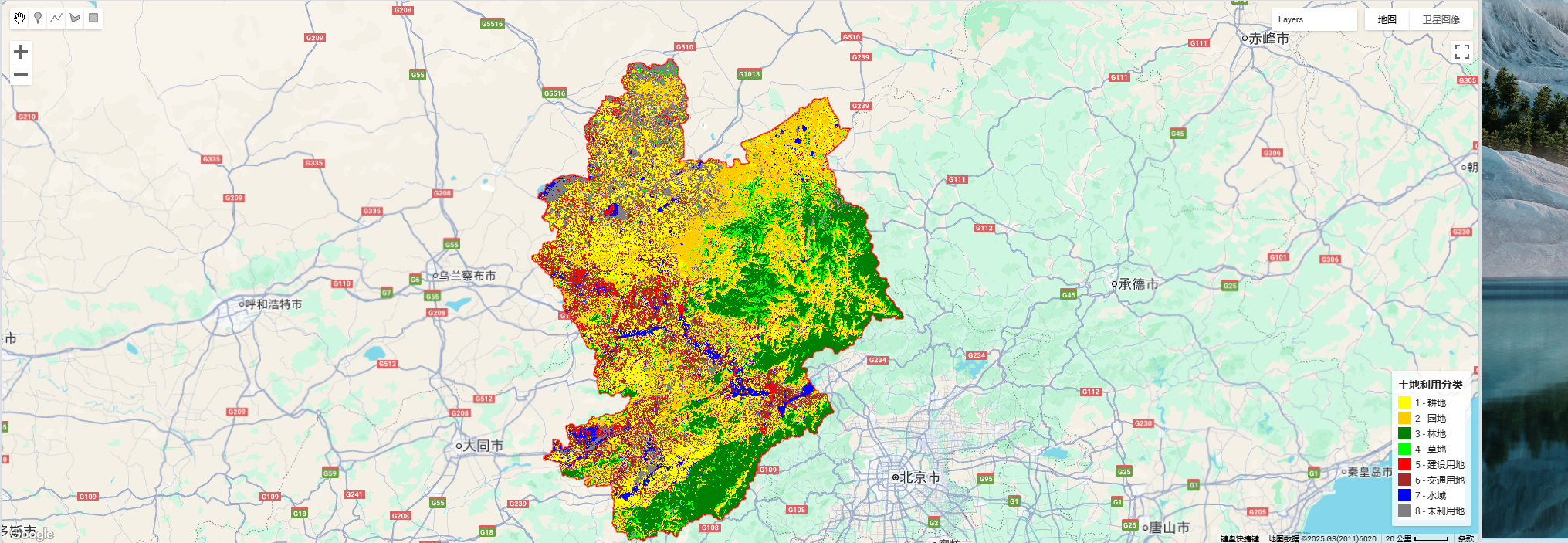
我这里用的数据是landset5，因为是90、95、05的数据，然后用的gee，样点的属性是landcover、lb，前者是1-8的值，后者对应地类名称，下面直接给代码
如果是landset8需要改一下波段值
样点的选择可以找开源的lucc数据来作为辅助

代码分享

查询对应区域的数据

// projects/ee-lth19981023/assets/zjk
//选择需要裁剪的矢量数据 
var cc = ee.FeatureCollection("projects/ee-lth19981023/assets/zjk");

// 去云函数 
function maskL8sr(image) {
  var cloudShadowBitMask = (1 << 3);
  var cloudsBitMask = (1 << 5);
  var qa = image.select('QA_PIXEL');
  var mask = qa.bitwiseAnd(cloudShadowBitMask).eq(0)
                 .and(qa.bitwiseAnd(cloudsBitMask).eq(0));
  return image.updateMask(mask);
}

// 选择并合并影像
var cc1995 = ee.ImageCollection('LANDSAT/LT05/C02/T1_L2')
                  .filterDate('2005-01-01', '2005-12-31')
                  .filterBounds(cc)
                  .map(maskL8sr)
                  .median()       // 按时间合成
                  .clip(cc);      // 裁剪到边界

// 强制转换成单一 mosaicked 影像
var final_img = cc1995.selfMask();  // 把无效值去掉，避免空洞

// 显示结果
Map.addLayer(final_img, {bands: ['SR_B5','SR_B4','SR_B3'], min: 0, max: 20000}, 'Landsat5_2005');

// 设置边界样式
var styling = {
  color: 'FF0000',
  fillColor: '00000000',
  width: 2
};
Map.addLayer(cc.style(styling), {}, "Boundary - No Fill");

// 导出到 Google Drive（单幅掩膜后影像）
Export.image.toDrive({
  image: final_img,
  description: 'Landsat5_2005_ZJK',
  folder: 'GEE_exports',
  scale: 30,
  region: cc.geometry(),
  crs: 'EPSG:32650',
  maxPixels: 1e13
});

分类代码

// ================== 1. 加载矢量边界 ==================
var cc = ee.FeatureCollection("projects/ee-lth19981023/assets/zjk");

// ================== 2. 加载样本点 ==================
var samplePoints = ee.FeatureCollection("projects/ee-lth19981023/assets/ls2005");
print('Sample Points Collection:', samplePoints);

// ================== 3. 去云函数（适用于 Landsat 5 C02）==================
function maskL5sr(image) {
  var qaMask = image.select('QA_PIXEL').bitwiseAnd(parseInt('11111', 2)).eq(0);
  var saturationMask = image.select('QA_RADSAT').eq(0);
  var mask = qaMask.and(saturationMask);
  return image.updateMask(mask).divide(10000); // 缩放到 0-1
}

// ================== 4. 加载影像 ==================
var cc2019 = ee.ImageCollection('LANDSAT/LT05/C02/T1_L2')
                  .filterDate('1990-01-01', '1990-12-31')
                  .filterBounds(cc)
                  .map(maskL5sr)
                  .median()
                  .clip(cc);

// ================== 5. 计算指数（修正波段名）==================
// ✅ MNDWI: Green (B3) vs SWIR1 (B5)
var mndwi = cc2019.normalizedDifference(['SR_B3', 'SR_B5']).rename('MNDWI');

// ✅ NDBI: SWIR1 (B5) vs NIR (B4)
var ndbi = cc2019.normalizedDifference(['SR_B5', 'SR_B4']).rename('NDBI');

// ✅ NDVI: NIR (B4) vs Red (B3)
var ndvi = cc2019.normalizedDifference(['SR_B4', 'SR_B3']).rename('NDVI');

// 合并波段
var imageWithIndices = cc2019.addBands([ndvi, ndbi, mndwi]);

// ✅ 修正训练波段：没有 SR_B6，用 SR_B5 代替原意中的 SWIR1
var bands = ['SR_B2', 'SR_B3', 'SR_B4', 'SR_B5', 'SR_B7', 'MNDWI', 'NDBI', 'NDVI'];
// 注意：SR_B1 可选，这里保留常用波段

// ================== 6. 提取样本 ==================
var training = imageWithIndices.select(bands).sampleRegions({
  collection: samplePoints,
  properties: ['landcover'],
  scale: 30,
  geometries: true
});

// ================== 7. 划分训练/测试集 ==================
var withRandom = training.randomColumn('random');
var split = 0.7;
var trainingPartition = withRandom.filter(ee.Filter.lt('random', split));
var testingPartition = withRandom.filter(ee.Filter.gte('random', split));

print('Training set size:', trainingPartition.size());
print('Testing set size:', testingPartition.size());

// ================== 8. 训练分类器 ==================
var classifier = ee.Classifier.smileRandomForest(50)
  .train({
    features: trainingPartition,
    classProperty: 'landcover',
    inputProperties: bands
  });

// ================== 9. 分类 ==================
var classified = imageWithIndices.select(bands).classify(classifier);

// ================== 10. 精度评估 ==================
var test = testingPartition.classify(classifier);
var confusionMatrix = test.errorMatrix('landcover', 'classification');
print('Confusion Matrix', confusionMatrix);
print('Overall Accuracy', confusionMatrix.accuracy());
print('Kappa Coefficient', confusionMatrix.kappa());

// ================== 11. 可视化 ==================
Map.centerObject(cc, 8);

// 设置显示样式：color代表边界颜色；fillColor代表填充颜色
var styling = {
  color: 'FF0000', // 使用十六进制颜色代码表示纯红色边框
  fillColor: '00000000', // 完全透明的填充色（8位十六进制，包含透明度）
  width: 2 // 可选，指定边框宽度
};

// 假设'cc'是你的矢量边界变量
Map.addLayer(cc.style(styling), {}, "Boundary - No Fill");

// 8 类颜色示例（请根据你的类别调整）
var classPalette = [
  '#ffff00', // 1 耕地
  '#ffcc00', // 2 园地
  '#008000', // 3 林地
  '#00ff00', // 4 草地
  '#ff0000', // 5 建设用地
  '#a52a2a', // 6 交通用地
  '#0000ff', // 7 水域
  '#808080'  // 8 未利用地
];

// 添加分类图层
Map.addLayer(classified, {
  min: 1, 
  max: 8, 
  palette: classPalette
}, 'Land Cover');

// 可选：真彩色合成
Map.addLayer(cc2019, {bands: ['SR_B4', 'SR_B3', 'SR_B2'], min: 0, max: 0.3}, 'True Color', false);


// 定义类别和颜色
var legendDict = {
  1: {label: '耕地', color: '#ffff00'},
  2: {label: '园地', color: '#ffcc00'},
  3: {label: '林地', color: '#008000'},
  4: {label: '草地', color: '#00ff00'},
  5: {label: '建设用地', color: '#ff0000'},
  6: {label: '交通用地', color: '#a52a2a'},
  7: {label: '水域', color: '#0000ff'},
  8: {label: '未利用地', color: '#808080'}
};

// 创建 legend 面板
var legend = ui.Panel({
  style: {
    position: 'bottom-right',
    padding: '8px',
    backgroundColor: 'ffffffcc' // 半透明白底
  }
});

// 标题
legend.add(ui.Label({
  value: '土地利用分类',
  style: {fontWeight: 'bold', fontSize: '14px', margin: '0 0 6px 0', textAlign: 'center'}
}));

// 添加每个类别的颜色和文字
Object.keys(legendDict).forEach(function(key) {
  var entry = legendDict[key];
  var colorBox = ui.Label({
    style: {
      backgroundColor: entry.color,
      padding: '8px',
      margin: '0 6px 4px 0'
    }
  });
  
  var description = ui.Label({
    value: key + ' - ' + entry.label,
    style: {margin: '0 0 4px 0', fontSize: '12px'}
  });
  
  var row = ui.Panel({
    widgets: [colorBox, description],
    layout: ui.Panel.Layout.Flow('horizontal')
  });
  
  legend.add(row);
});

// 把 legend 添加到地图
Map.add(legend);
// ================== 12. 导出 ==================
Export.image.toDrive({
  image: classified,
  description: '1990_land_cover_classification',
  fileNamePrefix: '1990lc',
  scale: 30,
  region: cc.geometry(),
  crs: 'EPSG:32650',
  maxPixels: 1e13,
  fileFormat: 'GeoTIFF'
});

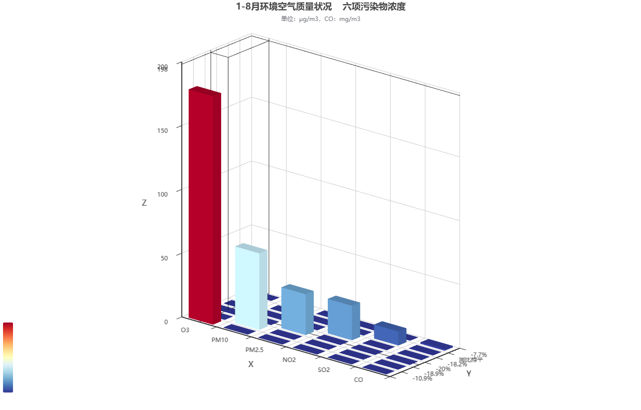
27-3d柱状图

制作网站https://www.hasgg.com/bar3d-chart-creation

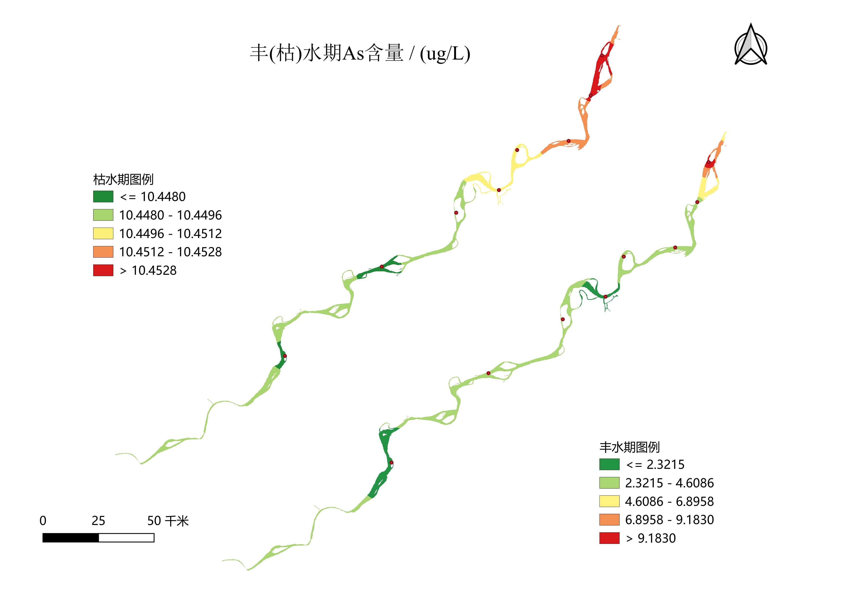
28-重金属含量长江安徽段出图

qgis出图，采样点矢量化，插值、掩膜、栅格符号化，然后就是出图三要素配置，这没什么好说的，下面只放一张
做了个批处理的qgis模型构建器

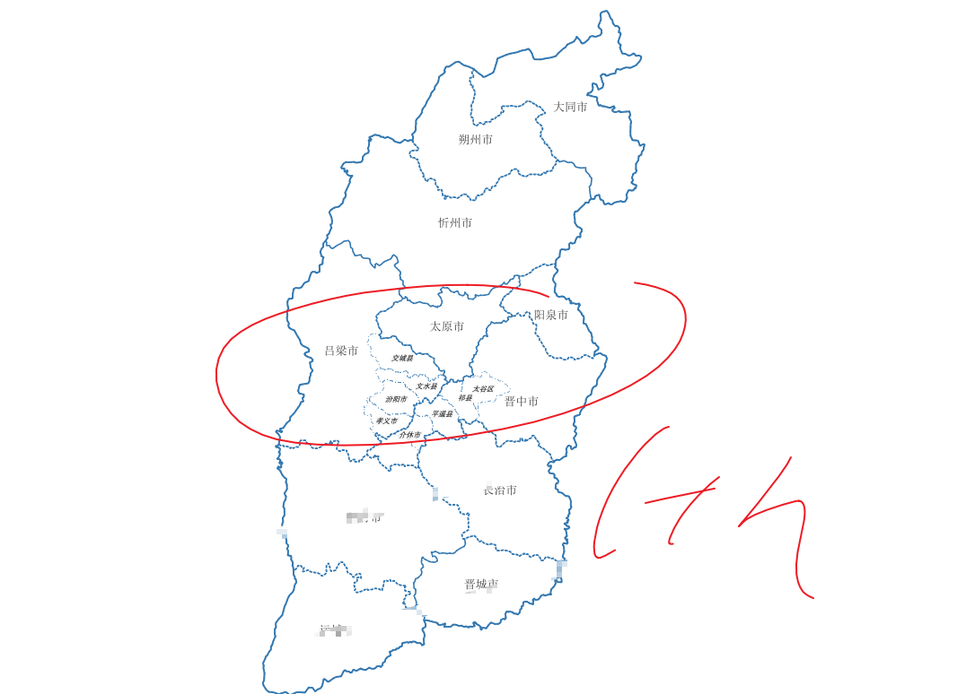
29-区位图

直接贴图

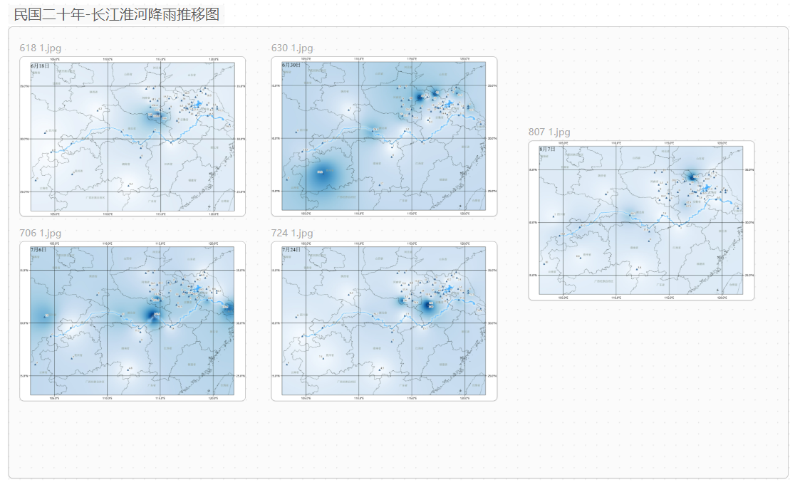
30-民国二十年-长江淮河降雨推移图

直接贴图

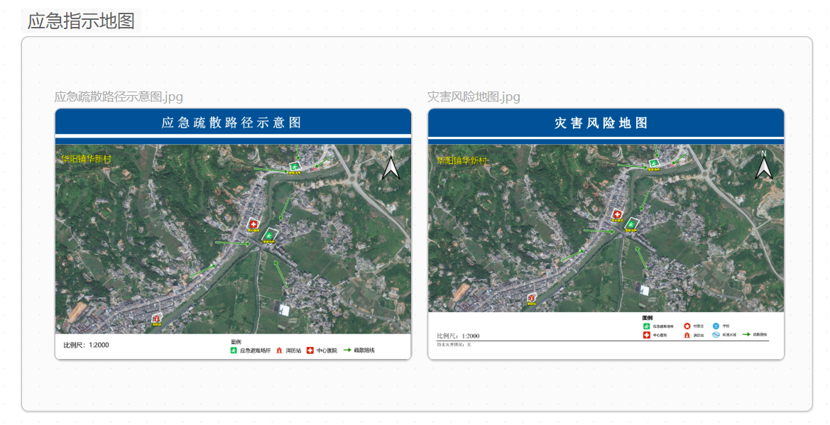
31-应急地图

直接贴图

32-郑州监测点

直接贴图

33-旅游线路+热力图

直接贴图

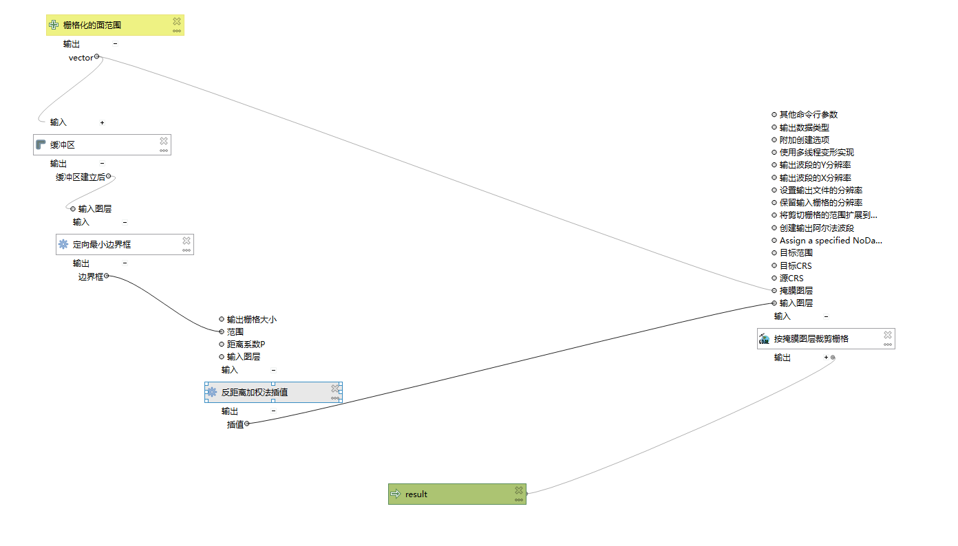
34-栅格补值

客户需求：
  一大一小两个栅格，大栅格包含小栅格，小栅格内的无效值补为自定义值，范围以大栅格有效值范围为准
拆解为：
  | expert 状态 | aspect 状态 | 结果                    |
  | --------- | --------- | --------------------- |
  | 有值        | 任意        | expert 值（保留小栅格）       |
  | NoData    | 有值        | 0（不是 aspect 值，而是固定 0） |
  | NoData    | NoData    | NoData                |

答案：
arcgispro版本
Con(IsNull("expert.asc"), Con(IsNull("aspect_extra31.asc"), "aspect_extra31.asc", 0), "expert.asc")
qgis版本
( ("expert@1" IS NULL) * 0 )                      -- 小栅格内部NoData → 填0（自定义值）
+ ( ("expert@1" IS NOT NULL) * "expert@1" )       -- 小栅格有值 → 保留原值
+ ( ("expert@1" IS NULL) * "aspect_extra31@1" )   -- 小栅格外部 → 补大栅格值

36-选址分析

客户需求：做配送中心的选址分析

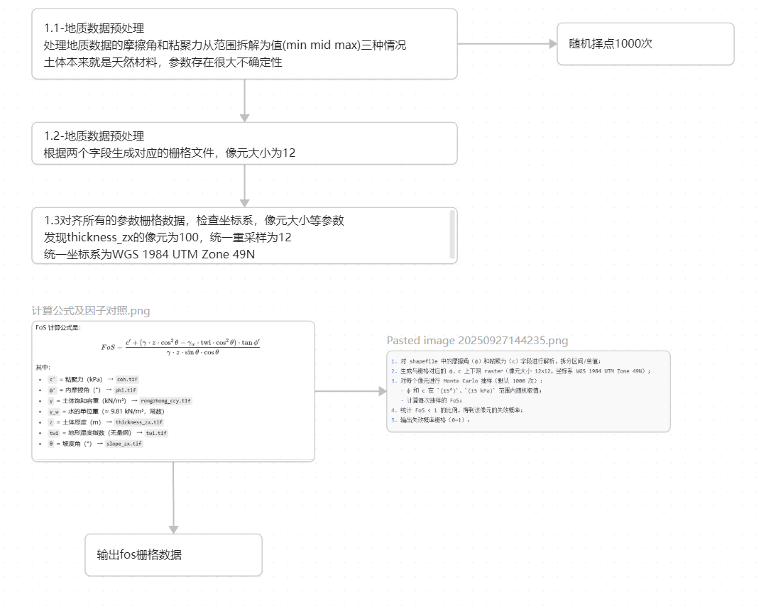
37-FOS滑坡失效概率计算

边（滑）坡工程设计中安全系数

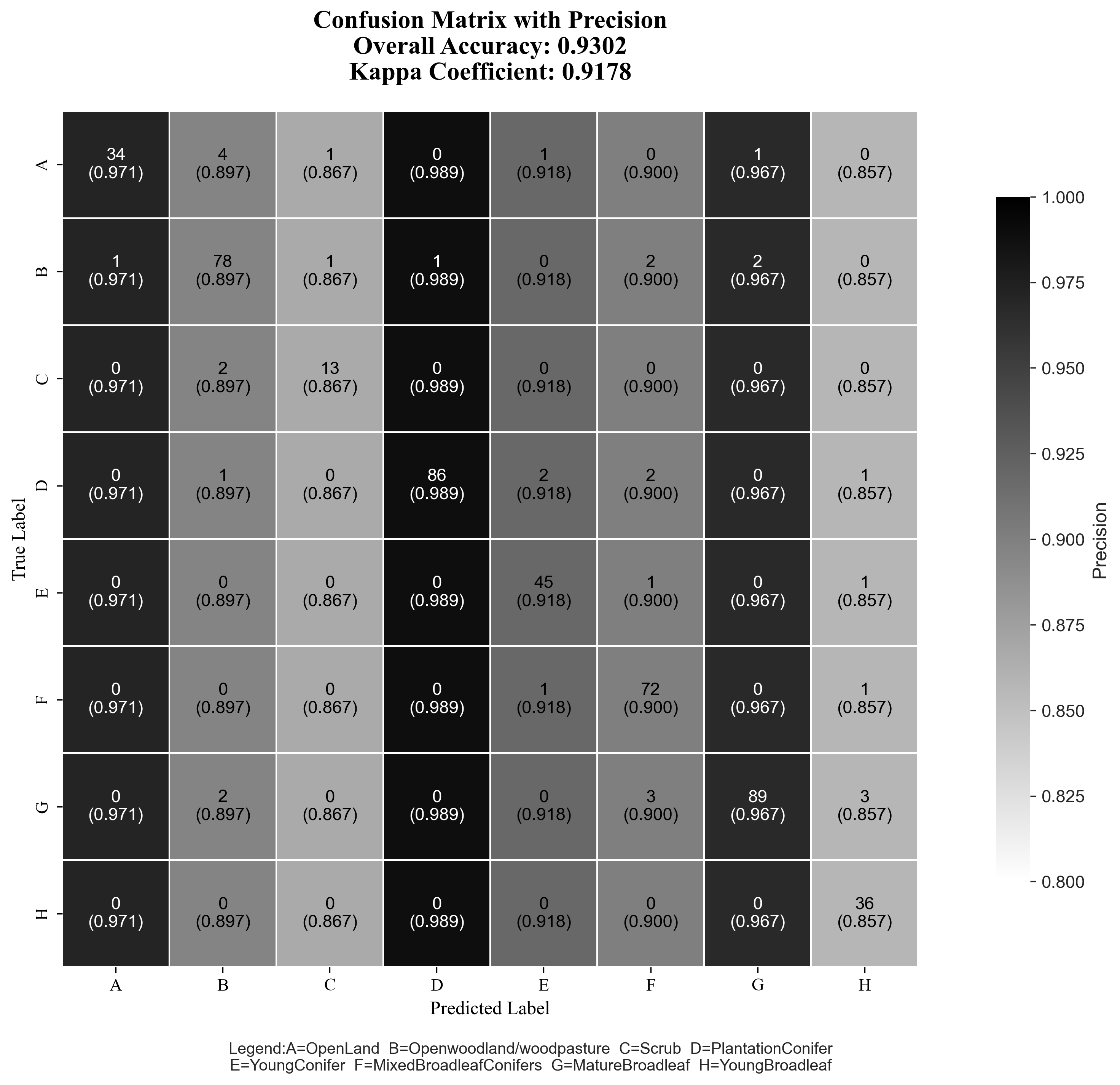
37-混淆矩阵

土地利用现状图、混淆矩阵0A&UA，土地利用转移桑基图及相关代码

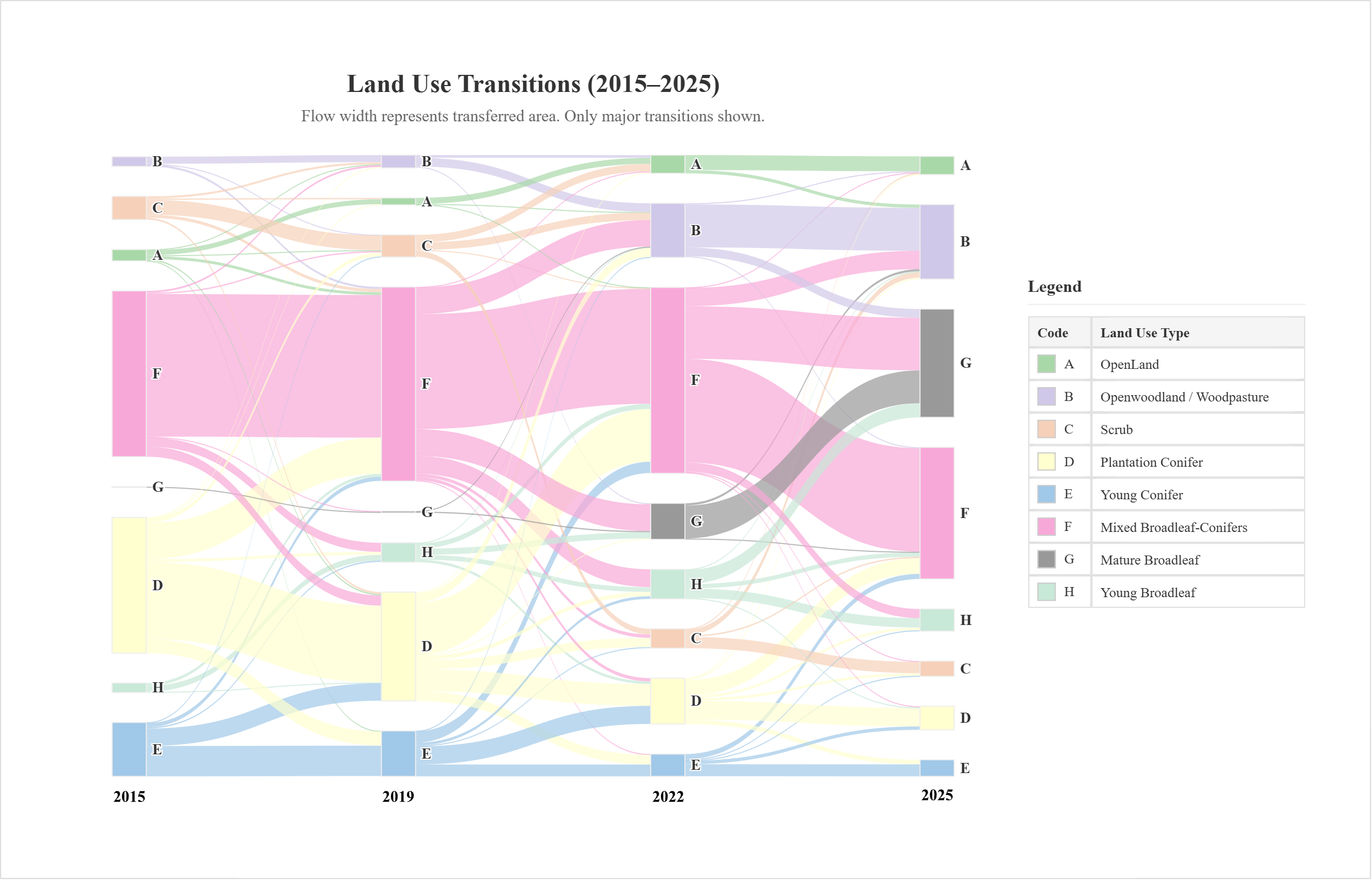
土地利用转移桑基图
<!DOCTYPE html>
<html lang="en">
<head>
   <meta charset="UTF-8">
   <title>Land Use Transitions (2015–2025)</title>
   <script src="https://cdn.jsdelivr.net/npm/echarts@5.4.3/dist/echarts.min.js"></script>
   <script src="https://cdn.jsdelivr.net/npm/papaparse@5.4.1/papaparse.min.js"></script>
   <script src="https://cdnjs.cloudflare.com/ajax/libs/html2canvas/1.4.1/html2canvas.min.js"></script>
   <style>
   body {
      font-family: 'Times New Roman', Times, serif;
      background-color: #f0f0f0;
      margin: 0; 
      color: #333;
      text-align: center;
   }

   /* 新增的外层容器用于控制导出时的白边和背景 */
   #export-wrapper {
      background-color: #ffffff; 
      box-sizing: content-box; 
      margin: 20px auto; 
      width: 1200px; 
   }

   .wrapper {
      /* 保持内部内容的布局和阴影 */
      padding: 20px;
      background-color: #ffffff;
      box-shadow: 0 2px 8px rgba(0,0,0,0.1);
   }

   .content-container {
      display: flex;
      align-items: center; /* 垂直居中对齐 */
      gap: 25px; 
   }

   #main {
      flex: 1;
      height: 700px;
   }

   #legend-container {
      flex-basis: 260px;
      flex-shrink: 0;
      text-align: left;
   }

   #legend-container h4 {
      margin-top: 5px;
      margin-bottom: 10px;
      font-size: 16px;
      border-bottom: 1px solid #eee;
      padding-bottom: 8px;
   }

   .legend-table {
      width: 100%;
      border-collapse: collapse;
      font-size: 13px;
   }

   .legend-table th, .legend-table td {
      border: 1px solid #e0e0e0;
      padding: 6px 8px;
      text-align: left;
   }

   .legend-table th {
      background-color: #f5f5f5;
   }

   .color-sample {
      display: inline-block;
      width: 15px;
      height: 15px;
      margin-right: 8px;
      border: 1px solid #ccc;
      vertical-align: middle;
   }

   #export-btn {
      margin-top: 15px;
      padding: 10px 20px;
      font-size: 16px;
      font-family: 'Times New Roman', Times, serif;
      cursor: pointer;
      border: 1px solid #3d85c6;
      background-color: #4a86e8;
      color: white;
      border-radius: 4px;
      transition: background-color 0.2s;
   }
   #export-btn:hover {
      background-color: #3d85c6;
   }
   </style>
</head>
<body>

<div id="export-wrapper">
   <div class="wrapper" id="capture-area">
   <div class="content-container">
      <div id="main"></div>
      <div id="legend-container">
      <h4>Legend</h4>
      <table class="legend-table">
         <thead>
         <tr>
            <th>Code</th>
            <th>Land Use Type</th>
         </tr>
         </thead>
         <tbody>
         <tr><td><div class="color-sample" style="background-color:#a8d8a8;"></div>A</td><td>OpenLand</td></tr>
         <tr><td><div class="color-sample" style="background-color:#d0c8e8;"></div>B</td><td>Openwoodland / Woodpasture</td></tr>
         <tr><td><div class="color-sample" style="background-color:#f6d0b8;"></div>C</td><td>Scrub</td></tr>
         <tr><td><div class="color-sample" style="background-color:#ffffd0;"></div>D</td><td>Plantation Conifer</td></tr>
         <tr><td><div class="color-sample" style="background-color:#a0c8e8;"></div>E</td><td>Young Conifer</td></tr>
         <tr><td><div class="color-sample" style="background-color:#f8a8d8;"></div>F</td><td>Mixed Broadleaf-Conifers</td></tr>
         <tr><td><div class="color-sample" style="background-color:#999999;"></div>G</td><td>Mature Broadleaf</td></tr>
         <tr><td><div class="color-sample" style="background-color:#c8e8d8;"></div>H</td><td>Young Broadleaf</td></tr>
         </tbody>
      </table>
      </div>
         </div>
   </div>
</div>

<button id="export-btn">Export as PNG</button>

<script>
// Color and label mapping
const colorMap = {
   'A': '#a8d8a8',   'B': '#d0c8e8',   'C': '#f6d0b8',   'D': '#ffffd0',
   'E': '#a0c8e8',   'F': '#f8a8d8',   'G': '#999999',   'H': '#c8e8d8'
};
const labelMap = { 0:'A', 1:'B', 2:'C', 3:'D', 4:'E', 5:'F', 6:'G', 7:'H' };
const years = ['2015', '2019', '2022', '2025'];
const fixedOrder = ['A','B','C','D','E','F','G','H'];

const myChart = echarts.init(document.getElementById('main'), null, {
   renderer: 'svg'
});

Papa.parse("土地利用转移.csv", {
   download: true,
   header: true,
   complete: function(results) {
   const data = results.data;
   const linkCounter = {};

   data.forEach(row => {
      const dn2015 = parseInt(row.DN2015), dn2019 = parseInt(row.DN2019),
         dn2022 = parseInt(row.DN2022), dn2025 = parseInt(row.DN2025);
      const area = parseFloat(row.area_last);
      if (isNaN(area)) return;

      const transitions = [
      { from: dn2015, to: dn2019, years: ['2015', '2019'] },
      { from: dn2019, to: dn2022, years: ['2019', '2022'] },
      { from: dn2022, to: dn2025, years: ['2022', '2025'] }
      ];
      transitions.forEach(t => {
      if (![0,1,2,3,4,5,6,7].includes(t.from) || ![0,1,2,3,4,5,6,7].includes(t.to)) return;
      const source = `${labelMap[t.from]} (${t.years[0]})`, target = `${labelMap[t.to]} (${t.years[1]})`;
      const key = `${source}→${target}`;
      linkCounter[key] = (linkCounter[key] || 0) + area;
      });
   });

   const nodesSet = new Set();
   const links = [];
   for (const [key, value] of Object.entries(linkCounter)) {
      const [source, target] = key.split('→');
      nodesSet.add(source);
      nodesSet.add(target);
      links.push({ source, target, value });
   }

   // ======================================================================
   // 强制排序和定位的修改部分
   // ======================================================================
   const nodes = [];
   const baseGap = 70; // 基础间隔
   
   // 1. 生成所有可能的节点（A到H），即使没有数据，以保持位置
   const allNodes = {};
   years.forEach(year => {
      fixedOrder.forEach((code, index) => {
         const name = `${code} (${year})`;
         // 使用 index * baseGap 来计算固定的 Y 轴位置，以保证 A 在最上，H 在最下
         allNodes[name] = { 
             name: name, 
             itemStyle: { color: colorMap[code] }, 
             // 强制设置 Y 轴位置（单位：像素）
             y: (index * baseGap), 
             fixed: true // 告诉 ECharts 不要移动这个节点
         };
      });
   });

   // 2. 过滤掉没有链接的节点，但保留其固定位置属性
   const existingNodeNames = new Set([...nodesSet]);
   
   Object.values(allNodes)
      .filter(node => existingNodeNames.has(node.name))
      .sort((a, b) => fixedOrder.indexOf(a.name[0]) - fixedOrder.indexOf(b.name[0])) // 排序以确保正确的布局计算
      .forEach(node => nodes.push(node));

   // ======================================================================
   // Sankey series option
   const sankeySeriesOption = {
      type: 'sankey', data: nodes, links: links,
      top: '12%', bottom: '5%',
      left: '5%', right: '5%',
      emphasis: { focus: 'adjacency' },
      lineStyle: { color: 'source', opacity: 0.7, curveness: 0.5, width: 1.5 },
      label: {
      position: 'right', fontSize: 14, fontWeight: 'bold', fontFamily: 'Times New Roman',
      formatter: params => params.name ? params.name.split(' ')[0] : ''
      },
      nodeWidth: 32, 
      nodeGap: 28,
      itemStyle: { borderWidth: 1, borderColor: '#eee' },
      // 保持 'none' 并依靠节点的 fixed: true 和 y 属性
      layout: 'none', 
      progressive: false
   };
    
   // 先设置一个包含标题和Sankey系列的option，以便ECharts计算布局
   const baseOption = {
        title: {
            text: 'Land Use Transitions (2015–2025)',
            subtext: 'Flow width represents transferred area. Only major transitions shown.',
            left: 'center',
            textStyle: { fontSize: 24, fontWeight: 'bold', fontFamily: 'Times New Roman', color: '#333' }, 
            subtextStyle: { fontSize: 15.5, fontFamily: 'Times New Roman', color: '#666' }
        },
        series: [sankeySeriesOption]
    };
   myChart.setOption(baseOption, true); 
   
   // 生成年份标签的 graphic 配置
   // 因为手动设置了 y 坐标，我们需要找到最底部的节点来放置年份标签
   const yearLabelsGraphics = [];
   const maxOrderIndex = fixedOrder.length - 1;
   const yearLabelY = (maxOrderIndex * baseGap) + sankeySeriesOption.nodeWidth + 25; // 根据最大 y 坐标计算

   // 重新获取布局信息来定位年份标签
   const sankeyLayout = myChart.getSeriesByType('sankey')[0];
   
   if (sankeyLayout && sankeyLayout.data.length > 0) {
      const yearColumnX = {}; 
      nodes.forEach(node => {
         const nodeLayout = myChart.convertToPixel({seriesIndex: 0}, node.name);
         if (nodeLayout) {
          const yearMatch = node.name.match(/\((\d{4})\)/);
          if (yearMatch) {
           const year = yearMatch[1];
           yearColumnX[year] = yearColumnX[year] || nodeLayout[0]; 
          }
         }
      });

      years.forEach(year => {
         if (yearColumnX[year]) {
          yearLabelsGraphics.push({
           type: 'text',
           left: yearColumnX[year], 
           top: yearLabelY,      
           style: {
            text: year,
            fill: '#333',
            fontSize: 16,
            fontWeight: 'bold',
            fontFamily: 'Times New Roman',
            textAlign: 'center'
           },
           z: 100 
          });
         }
      });
   }

   // 最终 option，包含标题、tooltip和graphic元素
   const finalOption = {
      ...baseOption, // 继承baseOption的title和series
      tooltip: {
      formatter: params => (params.data.value !== undefined)
         ? `<strong>${params.data.source}</strong> → <strong>${params.data.target}</strong><br/>Area: ${params.data.value.toFixed(0)} m²`
         : params.name,
      backgroundColor: 'white', borderColor: '#ccc', borderWidth: 1, padding: [10, 15],
      textStyle: { fontSize: 12, fontFamily: 'Times New Roman' }
      },
      graphic: yearLabelsGraphics // 添加年份标签
   };

   myChart.setOption(finalOption);
   },
   error: function(error) {
   console.error("CSV Parsing Error:", error);
   alert("Could not load data. Please check if the file exists.\nError: " + error.message);
   }
});

// 导出逻辑 (添加白边和外轮廓)
document.getElementById('export-btn').addEventListener('click', function () {
   const exportButton = this;
   const exportWrapper = document.getElementById('export-wrapper'); // 捕获外层容器
   const originalPadding = exportWrapper.style.padding;
   const originalBorder = exportWrapper.style.border;

   // 临时为导出区域添加额外的白边和边框
   const paddingForExport = 40; // 导出时四周增加的白边像素
   exportWrapper.style.padding = `${paddingForExport}px`;
   exportWrapper.style.border = '1px solid #ddd'; // 导出时添加外轮廓线

   exportButton.style.display = 'none'; // 隐藏导出按钮

   html2canvas(exportWrapper, {
   scale: 2, 
   logging: false, 
   useCORS: true, 
   backgroundColor: '#ffffff' // 确保背景是白色
   }).then(canvas => {
   const link = document.createElement('a');
   link.download = 'Land_Use_Transitions_Chart.png';
   link.href = canvas.toDataURL("image/png");
   link.click();
   link.remove();
   
   // 恢复原有样式
   exportWrapper.style.padding = originalPadding;
   exportWrapper.style.border = originalBorder;
   exportButton.style.display = 'block';
   }).catch(err => {
   console.error('Export failed:', err);
   
   // 确保在失败时也恢复样式
   exportWrapper.style.padding = originalPadding;
   exportWrapper.style.border = originalBorder;
   exportButton.style.display = 'block';
   });
});
</script>
</body>
</html>

# 混淆矩阵
import numpy as np
import matplotlib.pyplot as plt
import seaborn as sns
from sklearn.metrics import cohen_kappa_score

# === 设置字体为 Times New Roman ===
# 确保在运行环境中已安装 Times New Roman 字体，否则可能回退到默认字体
plt.rcParams['font.family'] = 'Times New Roman'
plt.rcParams['font.size'] = 12
plt.rcParams['axes.labelsize'] = 12
plt.rcParams['axes.titlesize'] = 16
plt.rcParams['xtick.labelsize'] = 11
plt.rcParams['ytick.labelsize'] = 11
plt.rcParams['legend.fontsize'] = 10

# === 混淆矩阵数据 ===
confusion_matrix_2025 = np.array([
    [34, 4, 1, 0, 1, 0, 1, 0],  # A - OpenLand
    [1, 78, 1, 1, 0, 2, 2, 0],  # B - Openwoodland/woodpasture
    [0, 2, 13, 0, 0, 0, 0, 0],  # C - Scrub
    [0, 1, 0, 86, 2, 2, 0, 1],  # D - PlantationConifer
    [0, 0, 0, 0, 45, 1, 0, 1],  # E - YoungConifer
    [0, 0, 0, 0, 1, 72, 0, 1],  # F - MixedBroadleafConifers
    [0, 2, 0, 0, 0, 3, 89, 3],  # G - MatureBroadleaf
    [0, 0, 0, 0, 0, 0, 0, 36]   # H - YoungBroadleaf
])


confusion_matrix_2015 = np.array([
    [130,   0,   1,   0,   0,   0,   0,   0],  # A (真实标签)
    [  4, 115,   0,   0,   0,   0,   0,   0],  # B
    [ 10,   1, 136,   0,   0,   0,   0,   0],  # C
    [  0,   7,   8, 129,   1,   2,   1,   3],  # D
    [  0,   0,   0,  14, 118,   1,   0,   1],  # E
    [  5,  26,   5,   7,   3, 128,   5,  14],  # F
    [  1,   0,   0,   0,   0,   0, 121,   0],  # G
    [  0,   0,   0,   2,   2,   4,   1, 131]   # H
])


confusion_matrix_2019 = np.array([
    [137,   1,   4,   0,   0,   0,   0,   0],  # A
    [  2, 124,   6,   0,   0,   1,   0,   1],  # B
    [  3,   3, 133,   1,   0,   1,   0,   0],  # C
    [  0,   4,   1, 136,  13,   6,   2,   4],  # D
    [  0,   0,   0,  11, 110,   0,   2,   2],  # E
    [  0,  16,   2,   2,   1, 126,   8,   7],  # F
    [  0,   0,   0,   0,   0,   0, 116,   0],  # G
    [  0,   0,   0,   0,   4,   4,   0, 135]  # H
])


confusion_matrix_2022 = np.array([
    [124,   2,   4,   1,   0,   0,   0,   0],  # A
    [  8, 117,   6,   0,   0,   2,   3,   0],  # B
    [  5,   1, 127,   1,   0,   2,   2,   0],  # C
    [  0,   4,   2, 133,   3,   1,   0,   4],  # D
    [  1,   0,   2,   3, 111,   0,   0,   2],  # E
    [  3,  18,   4,   5,   4, 120,   8,   8],  # F
    [  2,   2,   1,   1,   0,   2, 113,   2],  # G
    [  2,   1,   0,   0,   1,   2,   2, 129]  # H
])

confusion_matrix = confusion_matrix_2022














# === 字母对应完整名称 ===
label_names = {
    'A': 'OpenLand',
    'B': 'Openwoodland/woodpasture',
    'C': 'Scrub',
    'D': 'PlantationConifer',
    'E': 'YoungConifer',
    'F': 'MixedBroadleafConifers',
    'G': 'MatureBroadleaf',
    'H': 'YoungBroadleaf'
}

labels = list(label_names.keys())
total_samples = confusion_matrix.sum()

# --- 1. 计算 Producers Accuracy (PA) / Recall (行求和) ---
row_sums = confusion_matrix.sum(axis=1) # 真实标签的总和
producer_accuracies = [confusion_matrix[i, i] / row_sum if row_sum > 0 else 0.0 
                       for i, row_sum in enumerate(row_sums)]

# --- 2. 计算 Users Accuracy (UA) / Precision (列求和) ---
column_sums = confusion_matrix.sum(axis=0) # 预测标签的总和
user_accuracies = [confusion_matrix[i,i]/col_sum if col_sum > 0 else 0.0 
                  for i, col_sum in enumerate(column_sums)]

# --- 3. 计算 Overall Accuracy (OA) 和 Kappa 系数 ---
overall_accuracy = np.trace(confusion_matrix) / total_samples

# 构造真实标签和预测标签用于计算 Kappa
true_labels = []
pred_labels = []
for i in range(len(labels)):
    for j in range(len(labels)):
        count = confusion_matrix[i, j]
        true_labels.extend([i] * count)
        pred_labels.extend([j] * count)

kappa = cohen_kappa_score(true_labels, pred_labels)

# 打印所有结果
print(f"Total Samples: {total_samples}")
print(f"Overall Accuracy (OA): {overall_accuracy:.4f}")
print(f"Kappa Coefficient: {kappa:.4f}")
print("-" * 30)
print("Class | PA (Recall) | UA (Precision)")
print("-" * 30)
for i, label in enumerate(labels):
    print(f" {label}    |  {producer_accuracies[i]:.3f}     |  {user_accuracies[i]:.3f}")
print("-" * 30)


# --- 4. 可视化准备 ---

# 颜色矩阵：使用 UA/Precision 作为背景色
color_matrix = np.zeros_like(confusion_matrix, dtype=float)
for j in range(color_matrix.shape[1]):
    color_matrix[:, j] = user_accuracies[j]

# 标注文本：对角线显示 Count(PA, UA)，非对角线只显示 Count
annot = np.empty_like(confusion_matrix, dtype=object)
for i in range(confusion_matrix.shape[0]):
    for j in range(confusion_matrix.shape[1]):
        val = confusion_matrix[i, j]
        # 对角线元素：显示 Count 和 (PA, UA)
        if i == j:
            annot[i, j] = f"{val}\n(PA:{producer_accuracies[i]:.3f}\nUA:{user_accuracies[j]:.3f})"
        # 非对角线元素：只显示 Count
        else:
            annot[i, j] = f"{val}" 

# 自动根据背景亮度决定文字颜色
def get_text_color(val, vmin, vmax):
    norm_val = (val - vmin) / (vmax - vmin)
    return "black" if norm_val < 0.6 else "white"

text_colors = np.array([[get_text_color(user_accuracies[j], 0.8, 1.0) for j in range(8)] for _ in range(8)])

# === 5. 绘图 ===
fig, ax = plt.subplots(figsize=(14, 10))
sns.set_style("white")

hm = sns.heatmap(
    color_matrix, 
    annot=annot,
    fmt="",
    cmap="binary",  # 白→黑：小值白，大值黑
    cbar=True,
    cbar_kws={"shrink": 0.8, "label": "User's Accuracy (UA)", "pad": 0.02},
    square=True,
    linewidths=0.5,
    linecolor='white',
    xticklabels=labels,
    yticklabels=labels,
    annot_kws={"size": 10, "ha": 'center', "va": 'center'}, 
    ax=ax,
    vmin=0.8,
    vmax=1.0 
)

# 设置每个单元格的文字颜色
for i in range(8):
    for j in range(8):
        text_object = hm.texts[i * 8 + j]
        text_object.set_color(text_colors[i, j])

# 添加标题（包含 OA 和 Kappa）
title = f"Confusion Matrix with PA and UA\n" \
        f"Overall Accuracy (OA): {overall_accuracy:.4f}     Kappa Coefficient: {kappa:.4f}"
ax.set_title(title, fontsize=16, fontweight='bold', pad=20)
ax.set_xlabel("Predicted Label", fontsize=12)
ax.set_ylabel("True Label", fontsize=12)

# 图例
legend_text = "Legend:"
cols = 4
for i, (k, v) in enumerate(label_names.items()):
    if i % cols == 0:
        legend_text += f"\n{k}={v}"
    else:
        legend_text += f"  {k}={v}"

plt.figtext(0.55, 0.02, legend_text.strip(), ha='center', va='bottom', fontsize=10)

# 调整布局，留出图例空间
plt.tight_layout(rect=[0, 0.08, 1, 1])

# === 保存图像 ===
plt.savefig("full_classification_report_2025.png", dpi=300, bbox_inches='tight')

# plt.show()

68、兼职日志-Working with PostgreSQL in QGIS

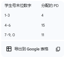
准备工作：确定分区

你的所有工作（包括回答问题和制作地图）都必须围绕一个特定的 TTS 规划区 (Planning District, PD) 进行。
学生号末尾数0  对应   PD=11

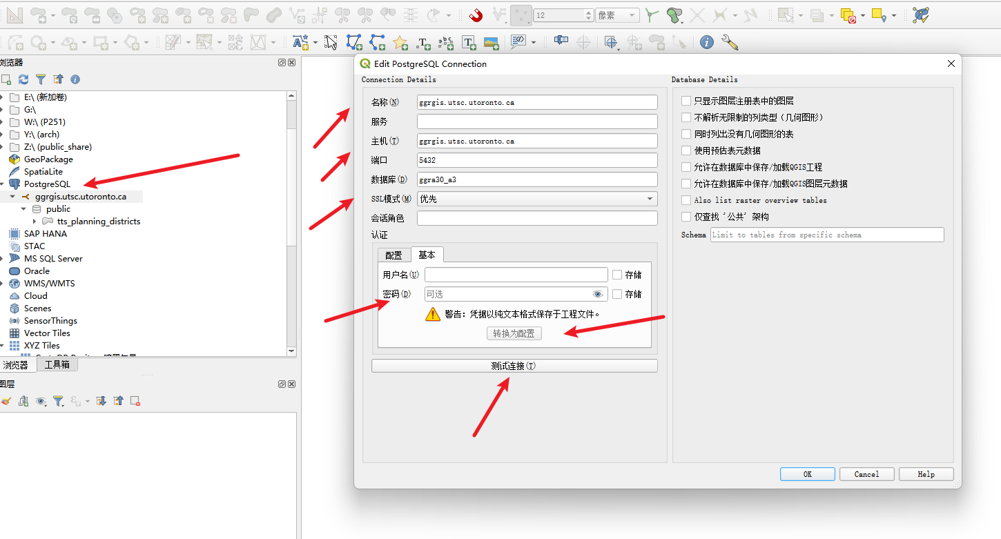
准备工作：链接数据库

数据源于“明天交通调查”（Transportation Tomorrow Surveys, TTS），包含以下两个主要表格：
tts_planning_districts：TTS 规划区的地理数据（矢量）图层 。
重要字段：pid (PD 编号) 、name (PD 名称) 、pop_pt_student (兼职学生人口) 、pop_ft_student (全职学生人口)  等。

tts_trip_counts：全职和兼职学生的每日通勤出行估计数 
重要字段：sur_year (调查年份) 、from_pid (出发地 PD 编号) 、to_pid (目的地 PD 编号) 、mode (出行方式) 、ntrips (估计的每日出行次数) 。

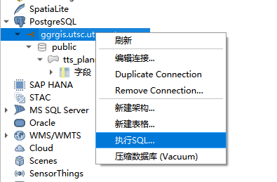
第一部分：SQL 查询问答 (Section 3.2)

右击数据库链接，点击执行sql，输入完sql后，点击Execute

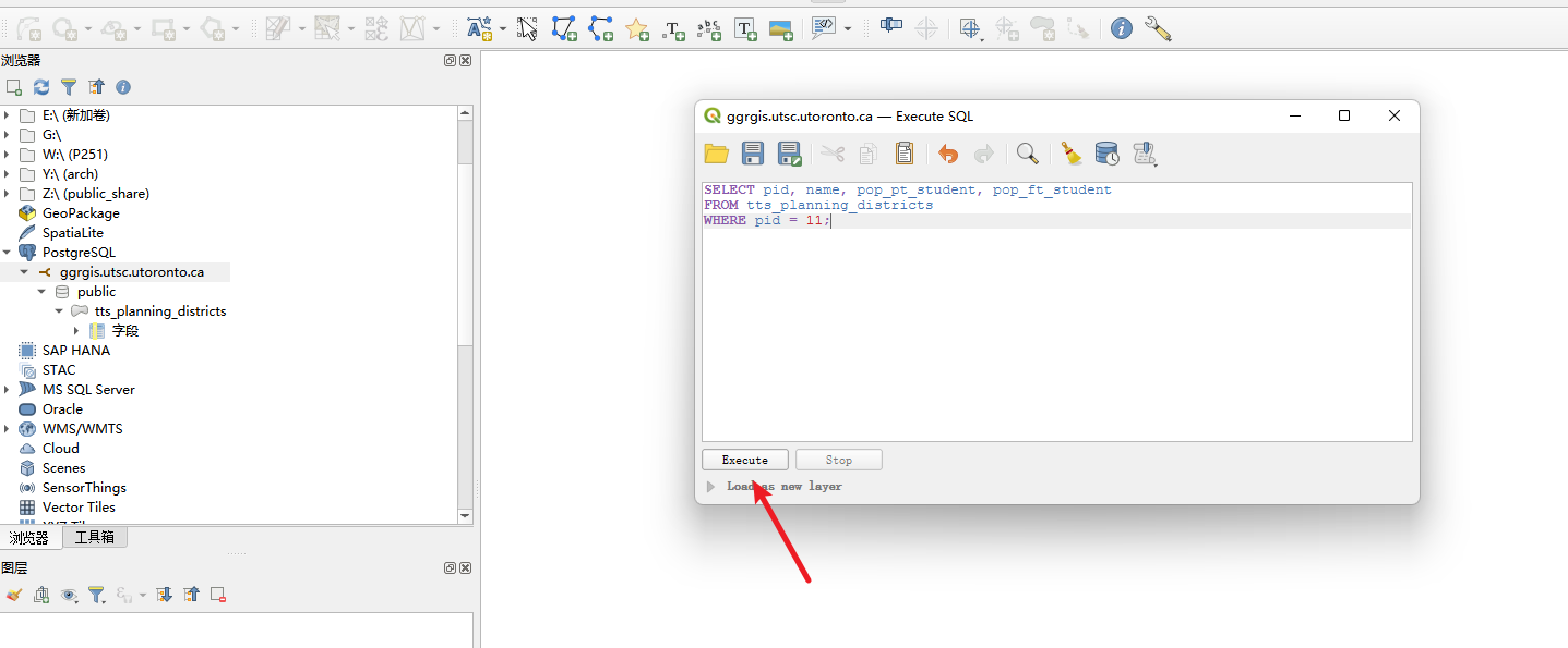
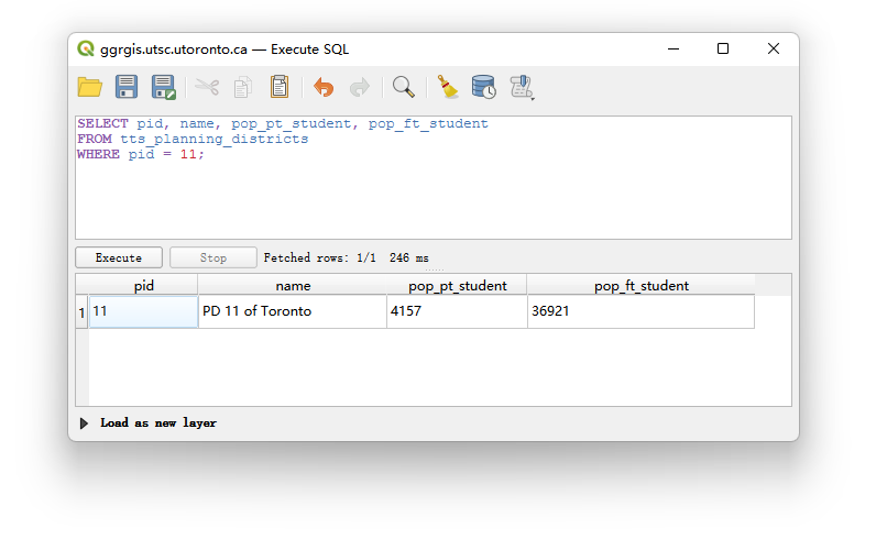
问题 1 (1 分): 列出你分配的 PD 的 pid、name、兼职学生人口 (pop_pt_student) 和全职学生人口 (pop_ft_student) 。

SELECT pid, name, pop_pt_student, pop_ft_student
FROM tts_planning_districts
WHERE pid = 11;

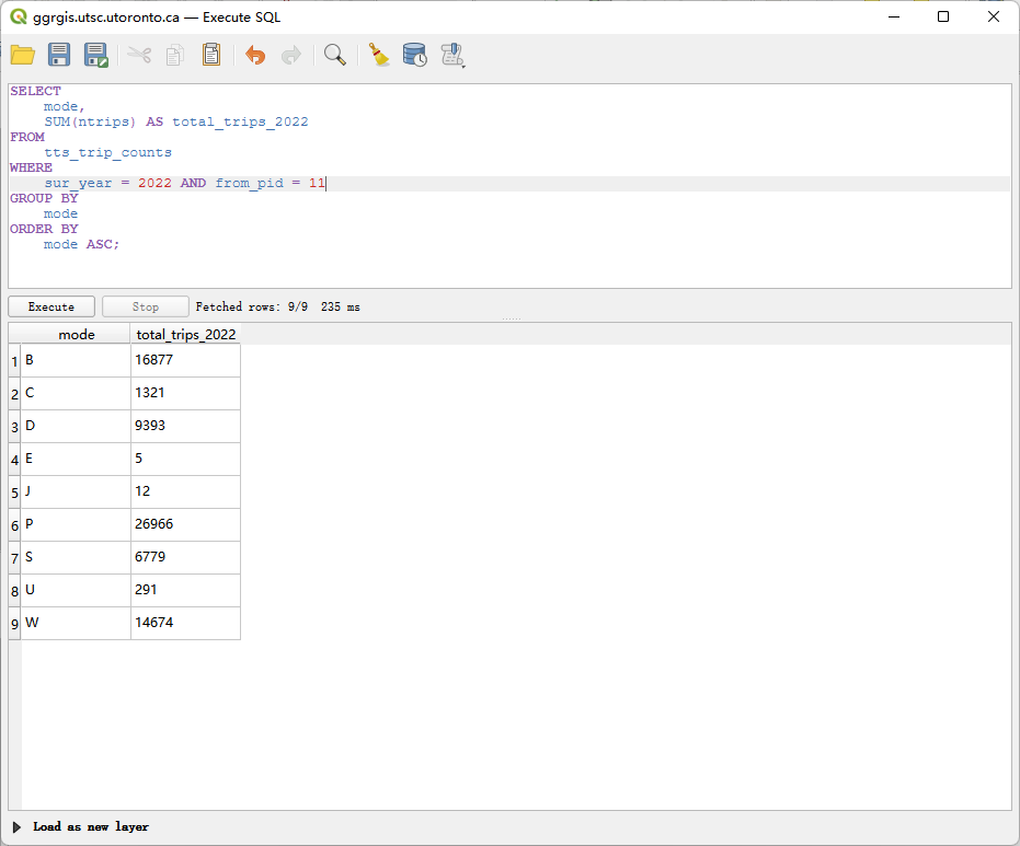
问题 2 (2 分): 统计 2022 年调查中，从你分配的 PD 出发（from_pid）的出行次数，结果需按出行方式 (mode) 分组小计 。

SELECT
    mode,
    SUM(ntrips) AS total_trips_2022
FROM
    tts_trip_counts
WHERE
    sur_year = 2022 AND from_pid = 11
GROUP BY
    mode
ORDER BY 
    mode ASC;

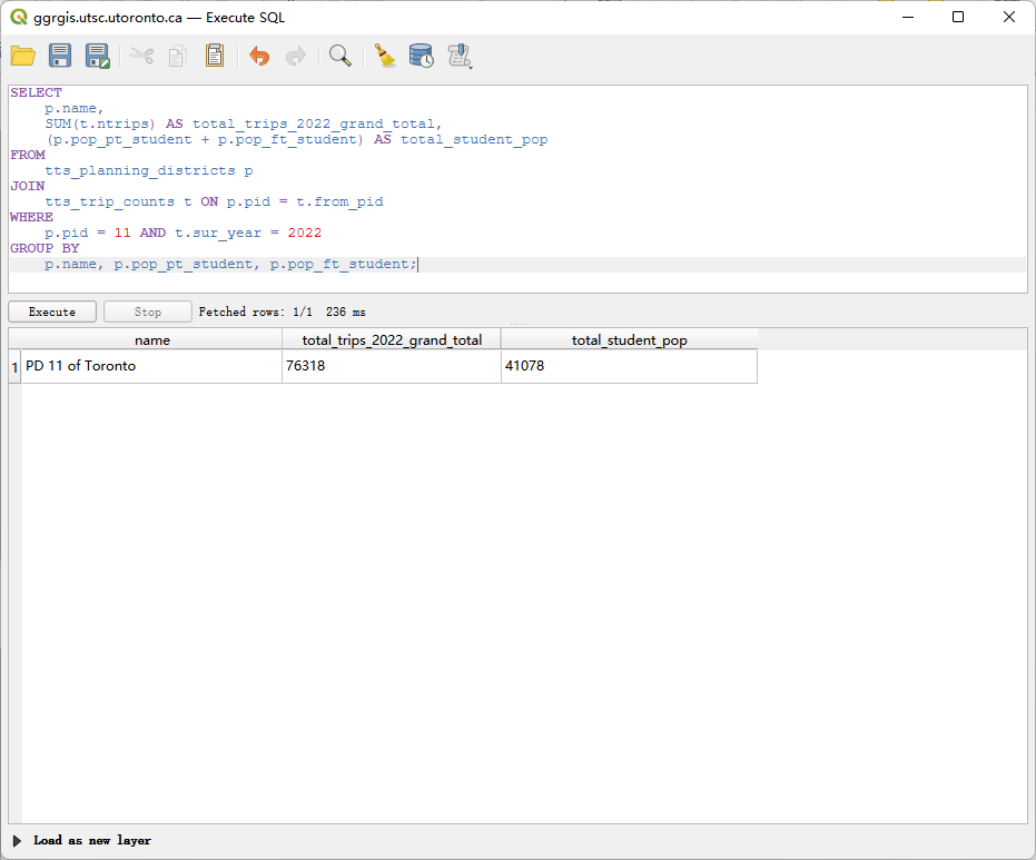
问题 3 (3 分): 创建一个查询来连接 tts_planning_districts 和 tts_trip_counts 表，结果需显示：你分配的 PD 的名称、2022 年调查中从该区出发的总出行次数，以及该区的已知学生总人口（兼职+全职）。同时，你需要解释这个结果与问题 2 的结果是否一致，并说明原因 。

SELECT
    p.name,
    SUM(t.ntrips) AS total_trips_2022_grand_total,
    (p.pop_pt_student + p.pop_ft_student) AS total_student_pop
FROM
    tts_planning_districts p
JOIN
    tts_trip_counts t ON p.pid = t.from_pid
WHERE
    p.pid = 11 AND t.sur_year = 2022
GROUP BY
    p.name, p.pop_pt_student, p.pop_ft_student;

解释这个结果与问题 2 的结果是否一致，并说明原因 ：
  经过计算结果是一致的。 问题 3 的 total_trips_2022_grand_total (160,042) 与将问题 2 中所有出行模式的总次数相加所得的总和 (160,042) 相等。这是因为这两个查询都是针对 2022 年，从 PD 11 出发的所有通勤记录进行汇总。问题 2 只是将总和按 mode 字段进行了分组，而问题 3 是直接计算了所有记录的总和，它们的操作集是相同的。

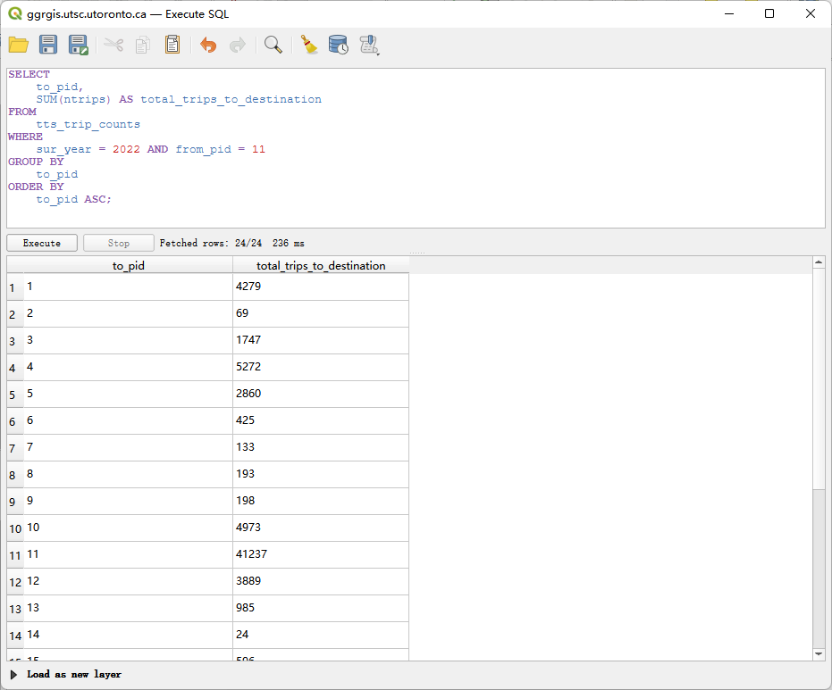
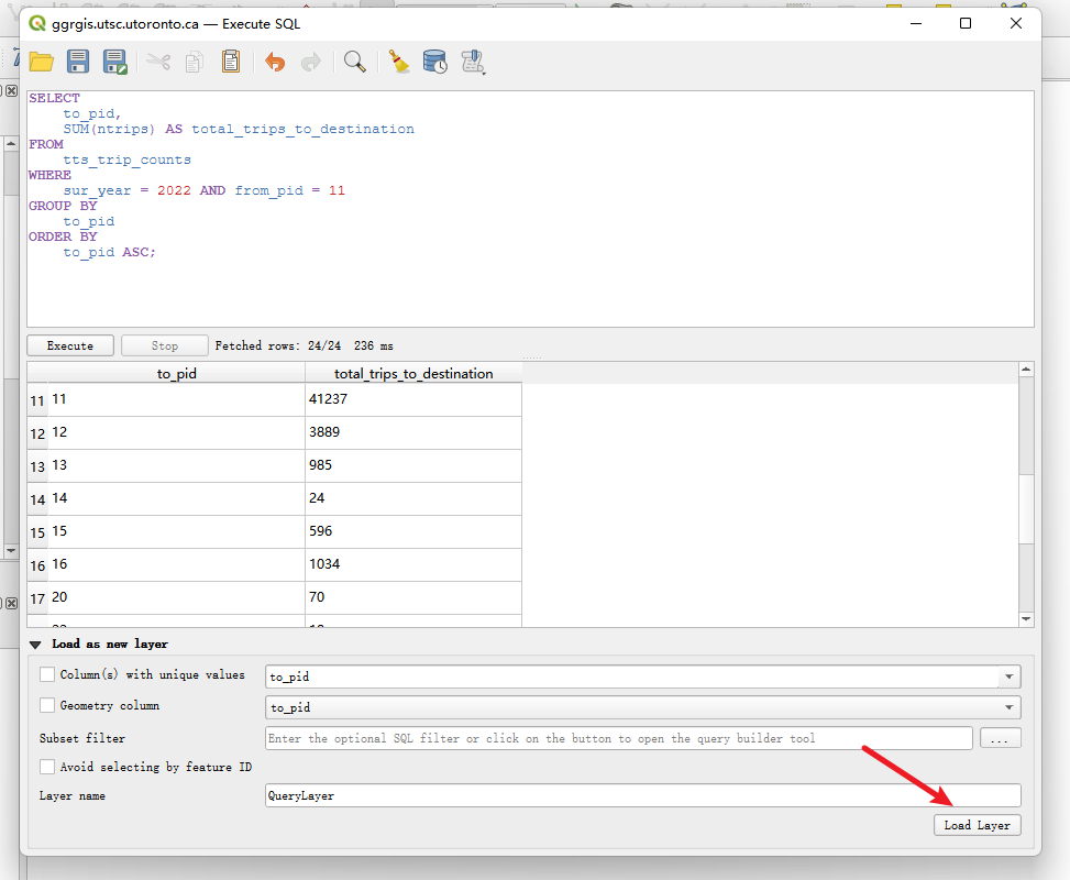
问题 4 (2 分): 统计 2022 年调查中，从你分配的 PD 出发，并以各个规划区为目的地 (to_pid) 的出行次数 。结果需显示目的地 PD 的 ID (to_pid) 和对应的总出行次数

SELECT
    to_pid,
    SUM(ntrips) AS total_trips_to_destination
FROM
    tts_trip_counts
WHERE
    sur_year = 2022 AND from_pid = 11
GROUP BY
    to_pid
ORDER BY
    to_pid ASC;

第二部分：创建查询图层并连接制图 (Section 3.3) (3 分)

使用问题 4 的查询结果，制作一张简单的地图 ：
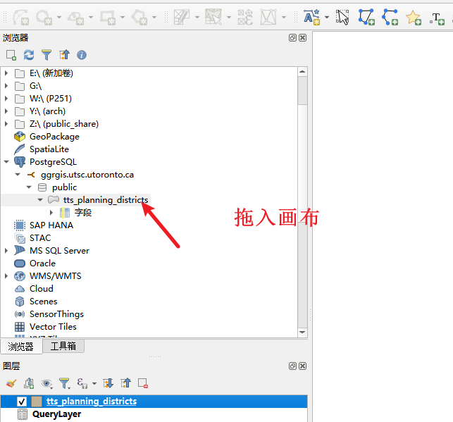
将问题 4 的查询结果作为新的图层，创建为一个 QGIS QueryLayer 。
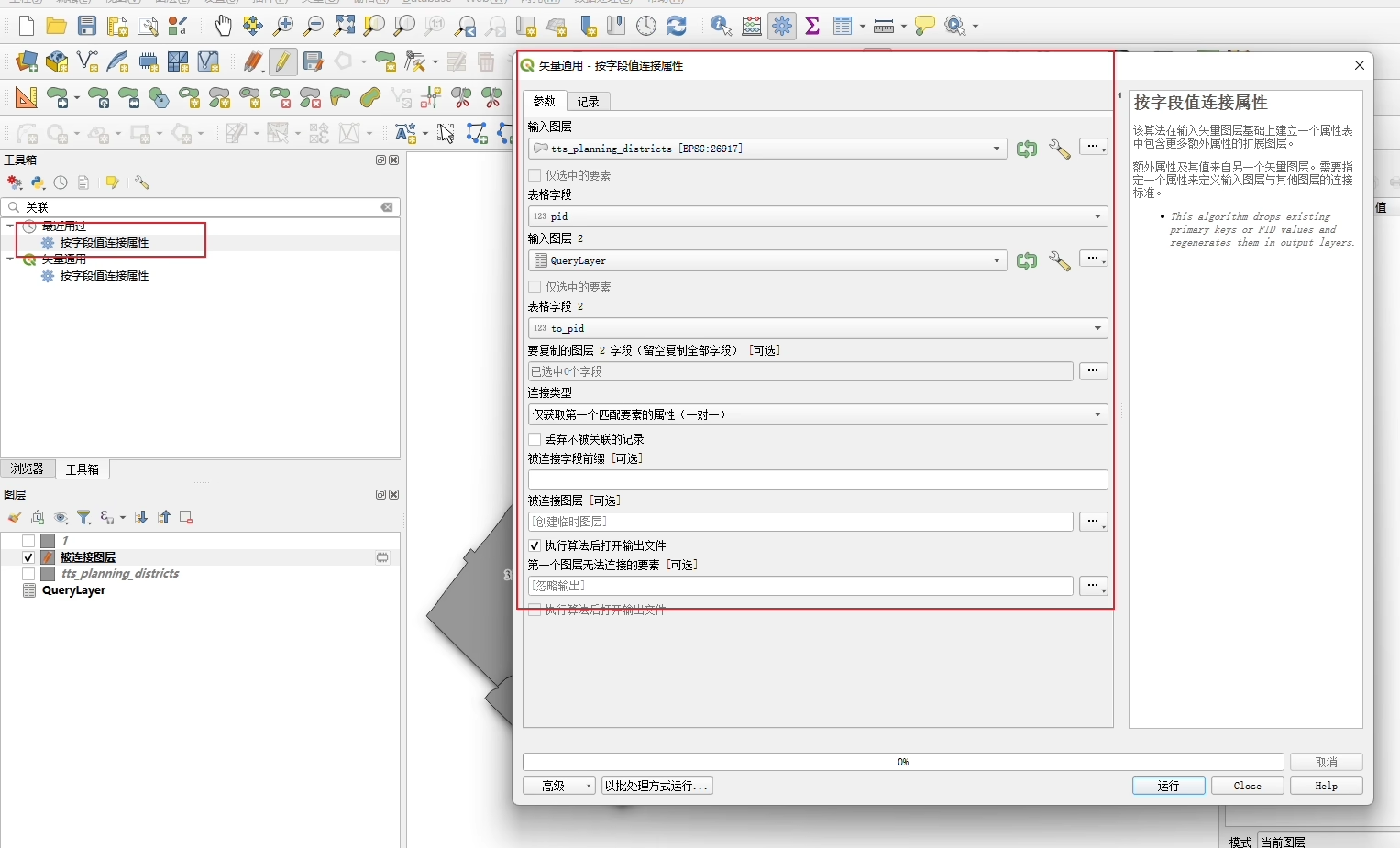
将此 QueryLayer 连接（Join）到 tts_planning_districts 图层上 。

加载查询结果，加载pg的矢量图层

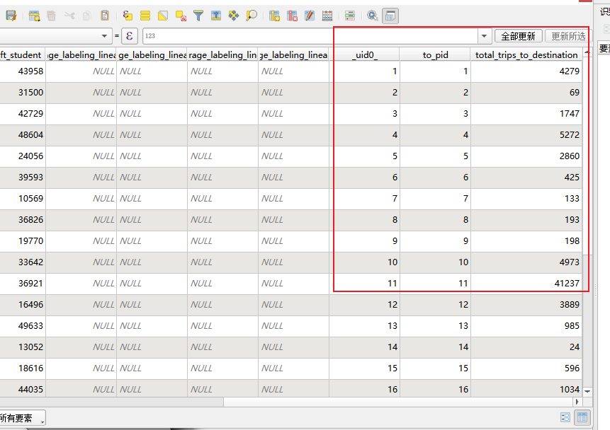
结果： 完成连接后，tts_planning_districts 图层的属性表中，将新增一列字段，其名称类似于 querylayer_total_trips_to_destination，该字段包含了从 PD 11 出发，到达该规划区的总出行次数。

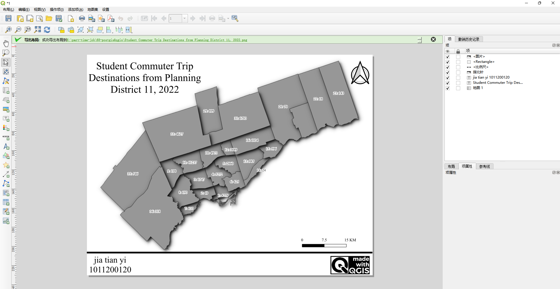
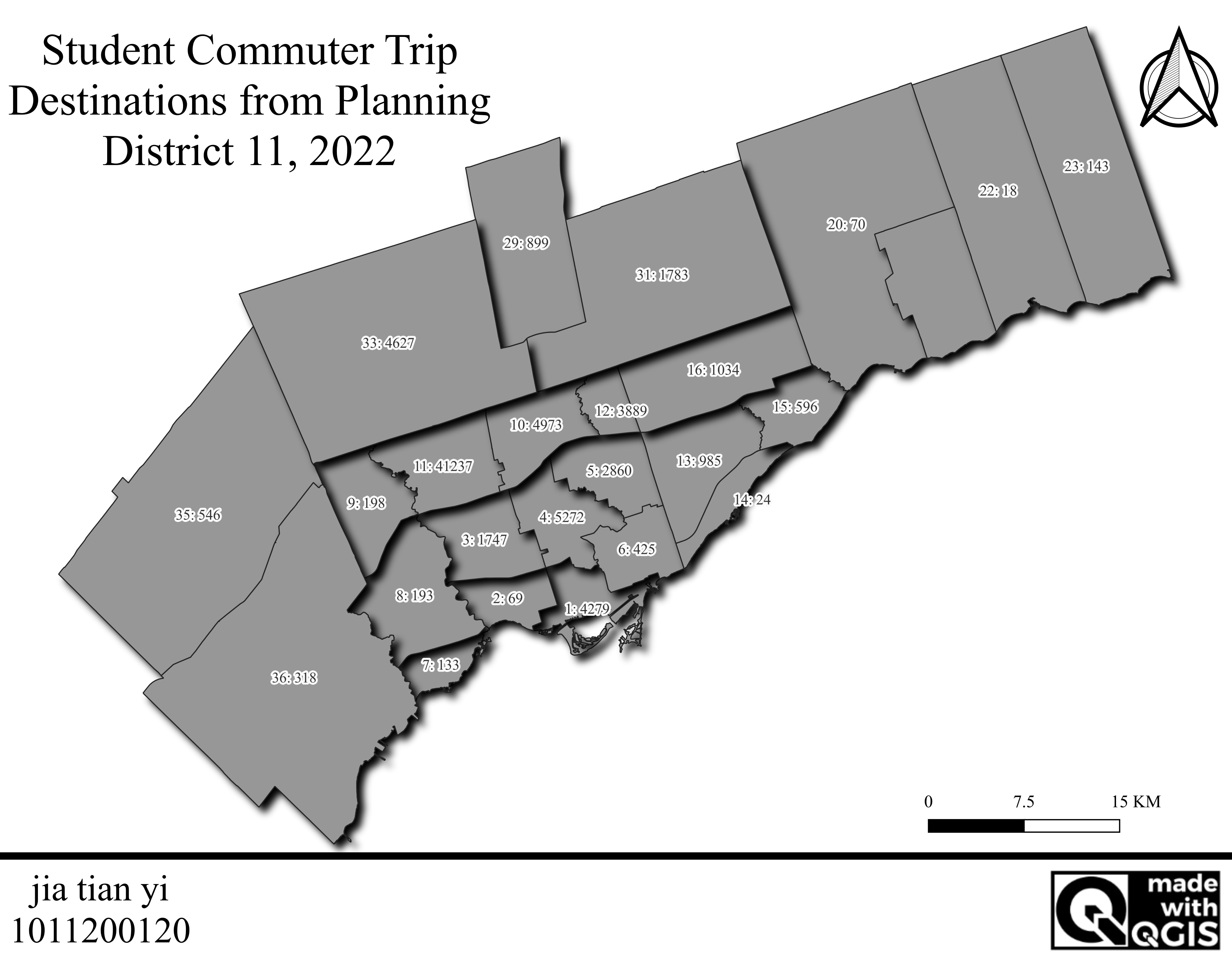
制作地图，要求如下 ：
地图只显示 tts_planning_districts 图层 。
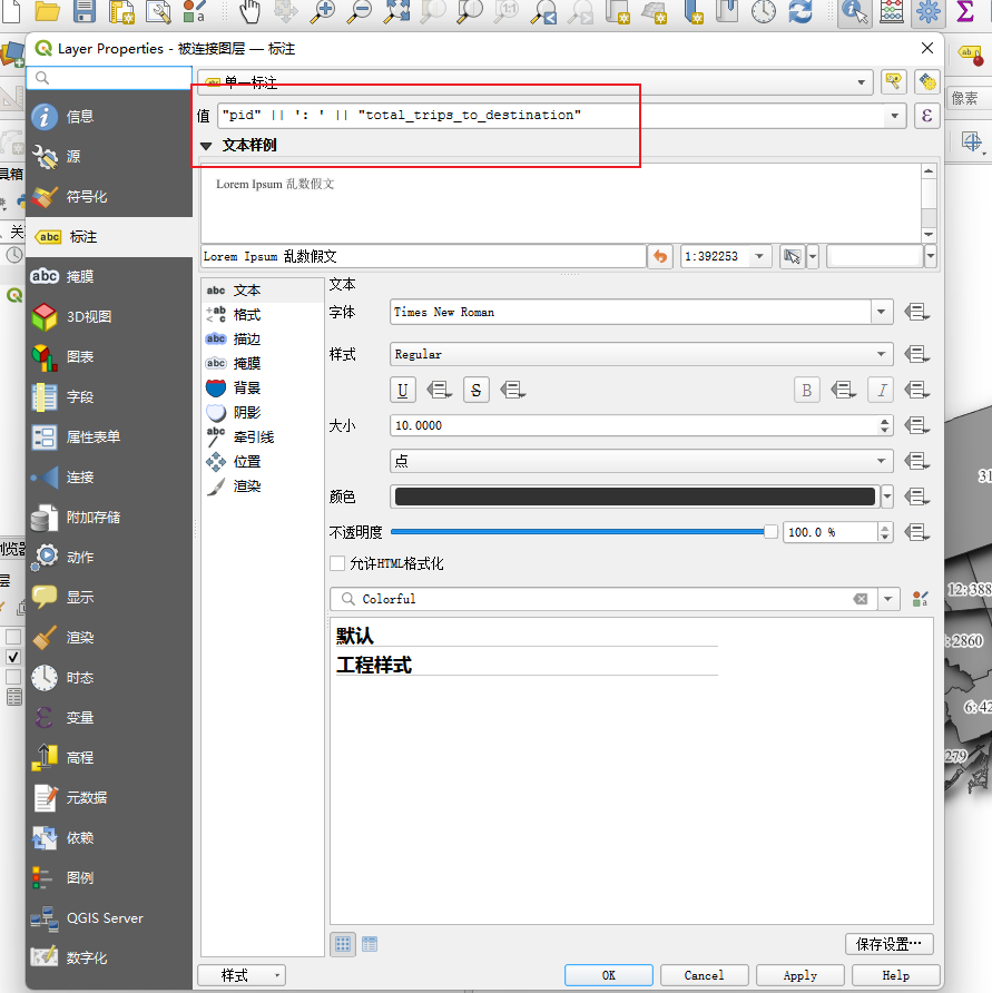
标注 (Label)：使用表达式标注每个规划区，内容为：PD ID + 冒号 + 到达该区的出行总数 。

示例：1: 23001 。
添加一个描述性的标题 。
添加一个文本框包含你的姓名和学号 。

先做标注
"pid" || ': ' || "total_trips_to_destination"

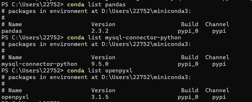
69、兼职日志-mysql&python出图

1、win安装mysql
安装包https://downloads.mysql.com/archives/installer/
安装步骤https://blog.csdn.net/mumiandeci/article/details/134520684
数据库连接工具https://www.hexhub.cn/

CREATE DATABASE IF NOT EXISTS database_name CHARACTER SET utf8mb4 
COLLATE utf8mb4_unicode_ci;


DROP TABLE IF EXISTS `spatial_database_nationwide`;
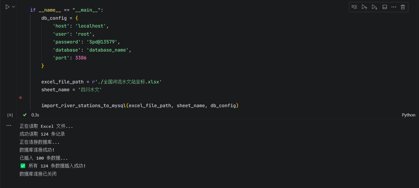
CREATE TABLE `spatial_database_nationwide` (
`id` INT NOT NULL AUTO_INCREMENT COMMENT '全国河流水文站坐标_全
国',
 `name` varchar(255) CHARACTER SET utf8mb4 COLLATE 
utf8mb4_0900_ai_ci NULL DEFAULT NULL COMMENT '水文站名字',
`point` point NULL COMMENT '存储点数据',
 PRIMARY KEY (`id`) USING BTREE
) ENGINE = InnoDB AUTO_INCREMENT = 63 CHARACTER SET = utf8mb4 
COLLATE = utf8mb4_0900_ai_ci ROW_FORMAT = Dynamic;

2、将四川水文Excel写入mysql空间数据库

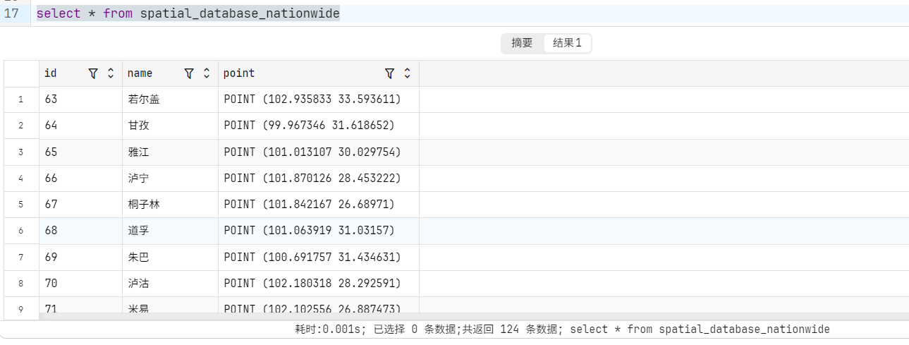
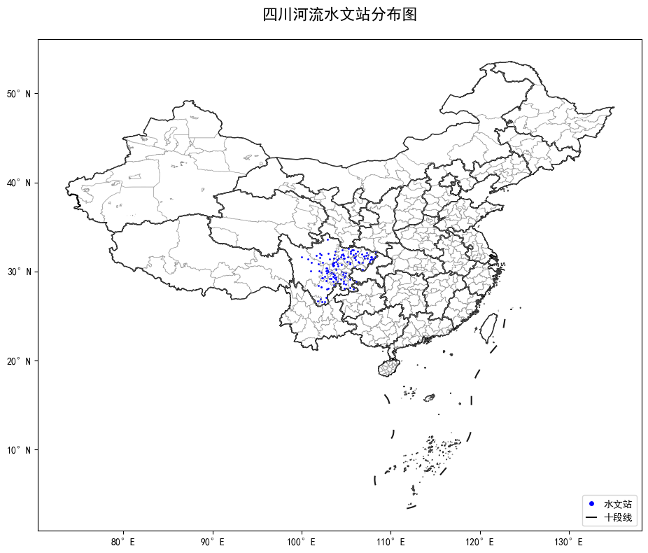
3、可视化四川水文站

70、兼职日志-GIS and Empirical Reasoning

详细步骤

1、登录并上传数据

1.1用账号密码登录
https://utoronto.maps.arcgis.com/home/index.html


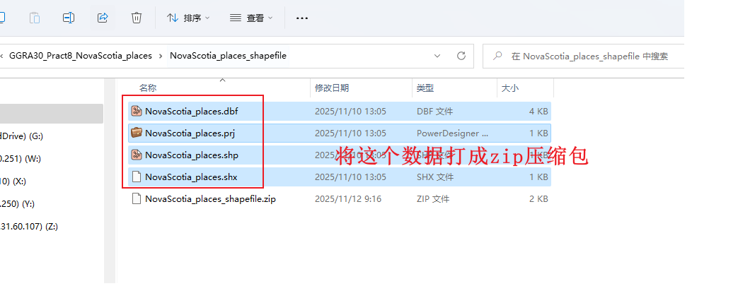
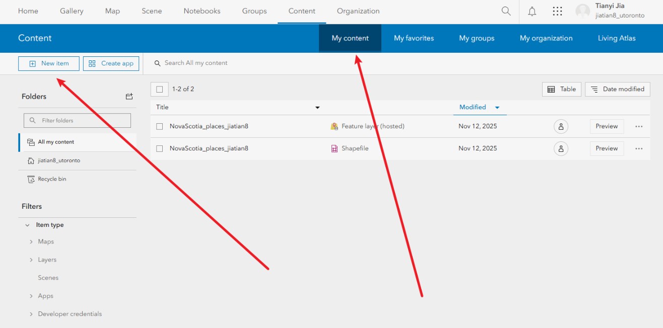
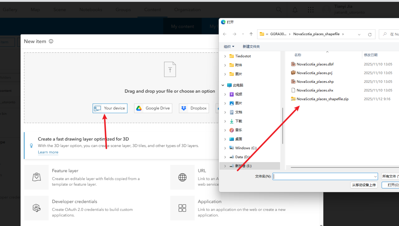
1.2上传关键NovaScotia_places.shp数据的压缩包
滑到网站最上方，点击content,点击new item,点击your device，然后上传自己的zip
然后默认选项create a hosted feature layer 点击next,
修改title为NovaScotia_places_jiatian8
然后点击save

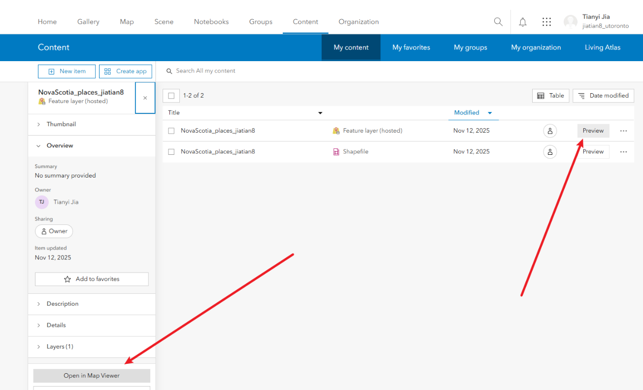
2、在地图中打开托管要素图层

2.1点击preview ,点击open in map viewer

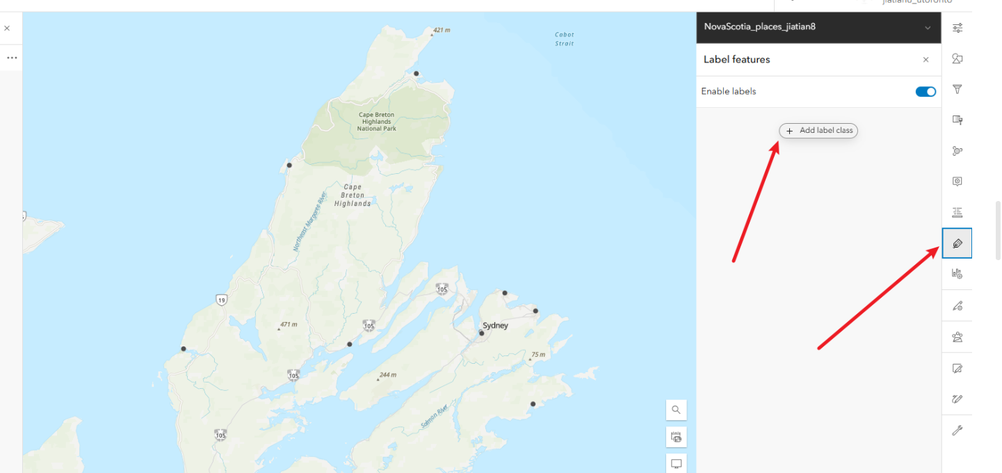
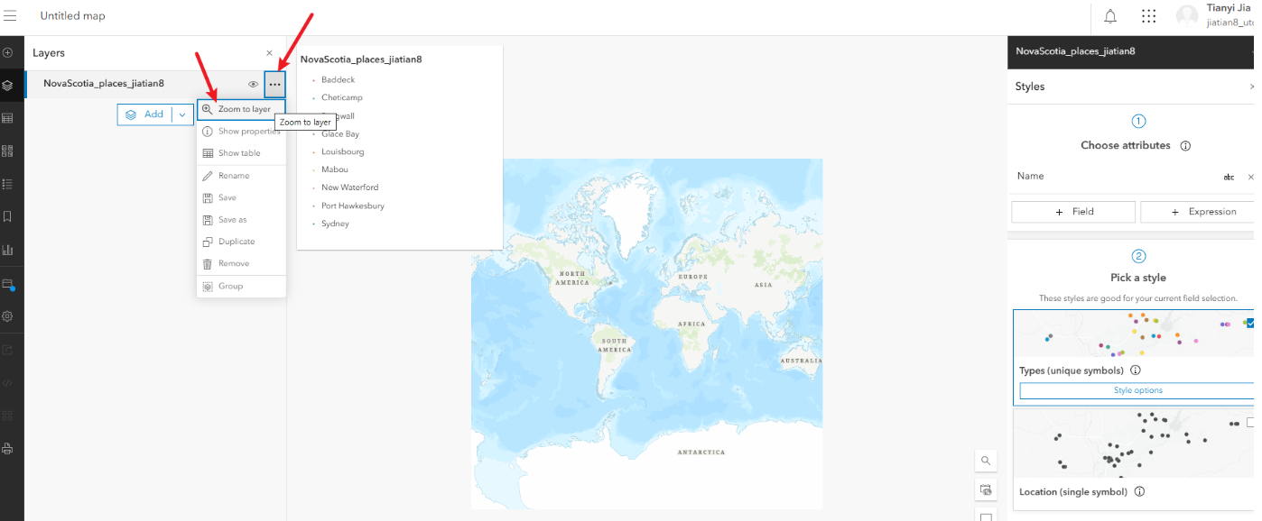
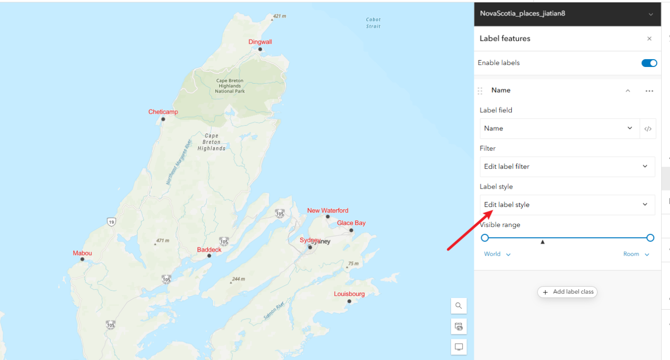
3、配置标签

3.1、点击右侧label选项。添加新标签
3.2、以name字段来可视化标签
3.3、缩放到图层查看配置情况
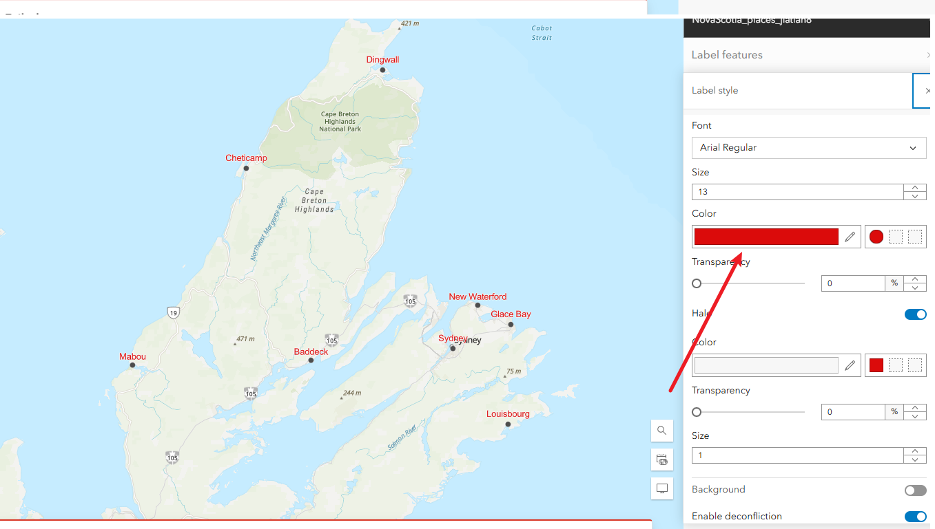
3.4、给标签改颜色，编辑标签属性，进去改成其他颜色，方便直观展示

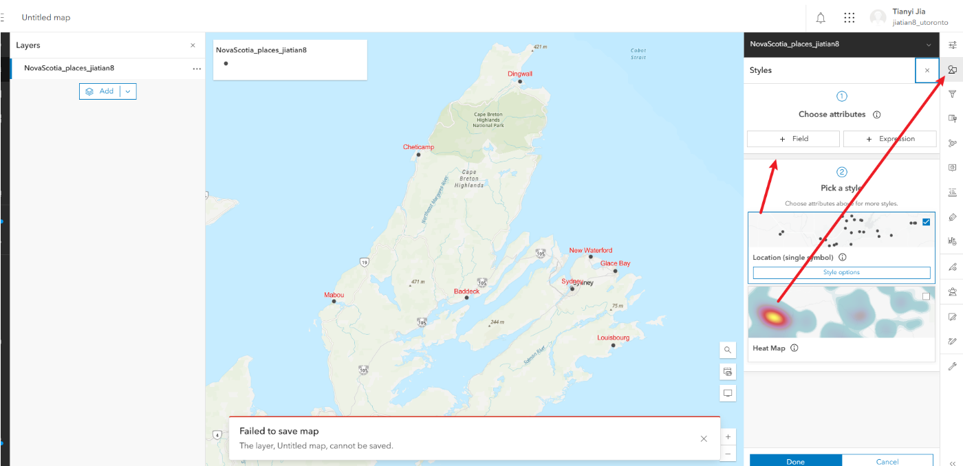
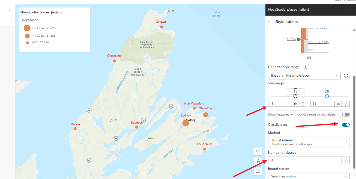
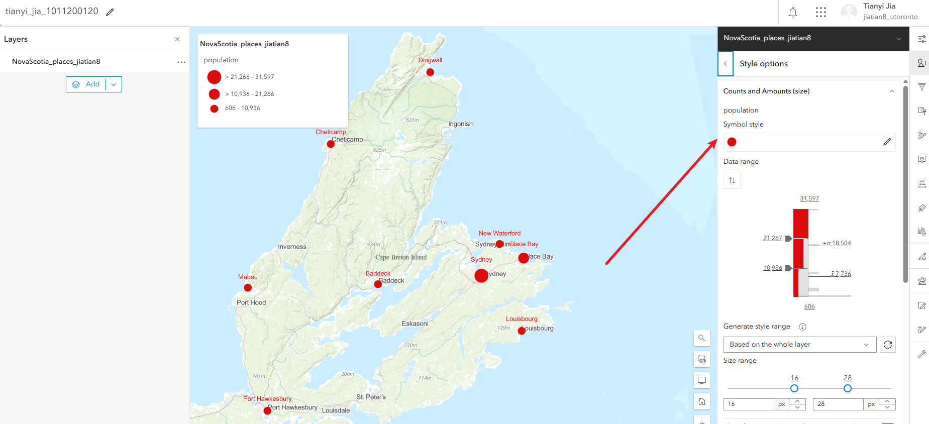
4、配置符号

3.1、点击右侧styles面板
3.2、以pop人口字段来可视化
3.3、点击这个style options,修改符号属性
3.4、工序按classify data,修改number of classes为3，修改最小的px改大一点，让小数值也可以清晰显示
3.5、往上滑，修改一下符号颜色symbol style,这里随便改一下不要是原本的颜色就可以
3.6、修改完成点击下方的done即可

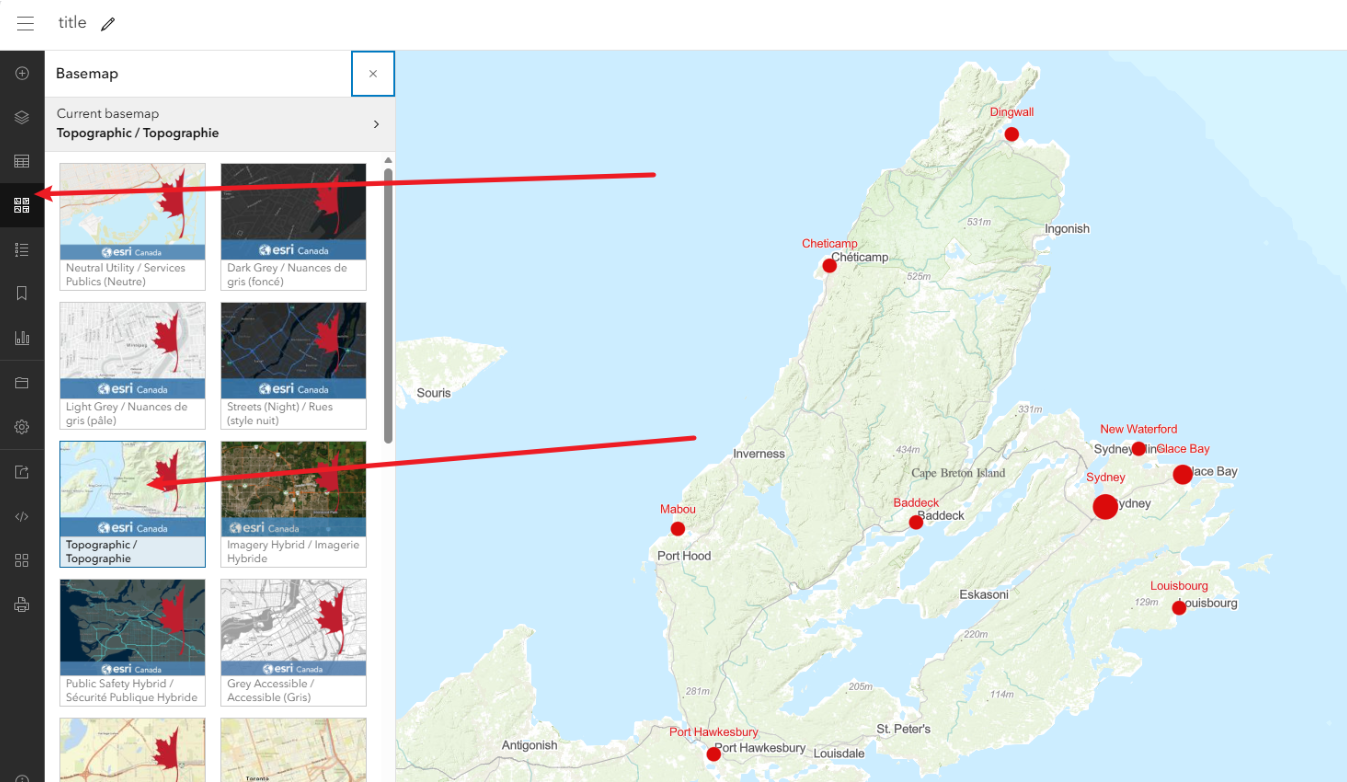
5、底图更换，另存为，共享

5.1、点击左侧的basemap，更换一个底图
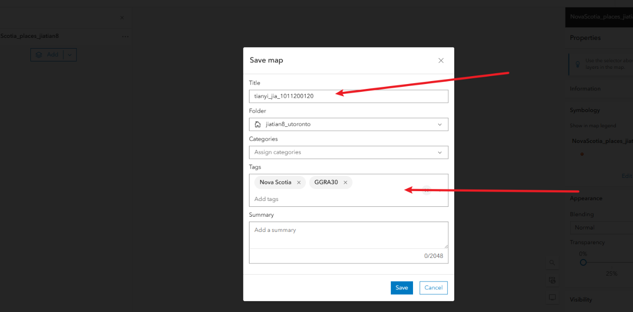
5.2、点击save as另存为
5.3、点击左侧的save and open 然后save as 输入一个title,包含学号姓名tianyi_jia_1011200120，tag标签随便写Nova Scotia,GGRA30然后点击save
5.4、回到最初的content,点击进入详情页面，然后点击分享，选组织然后save
5.5、回到地图中，点击左侧的分享，复制分享链接
最后的地图链接
https://arcg.is/1TiOTn4

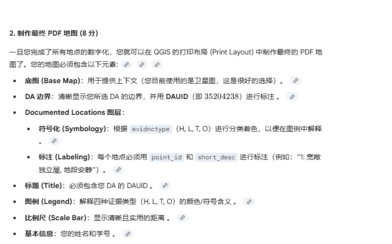
82、GGRA30_Assign4

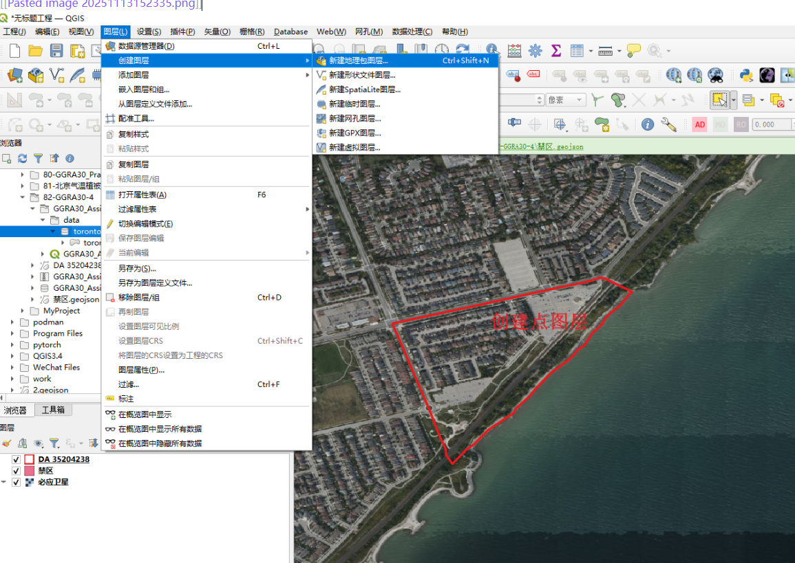
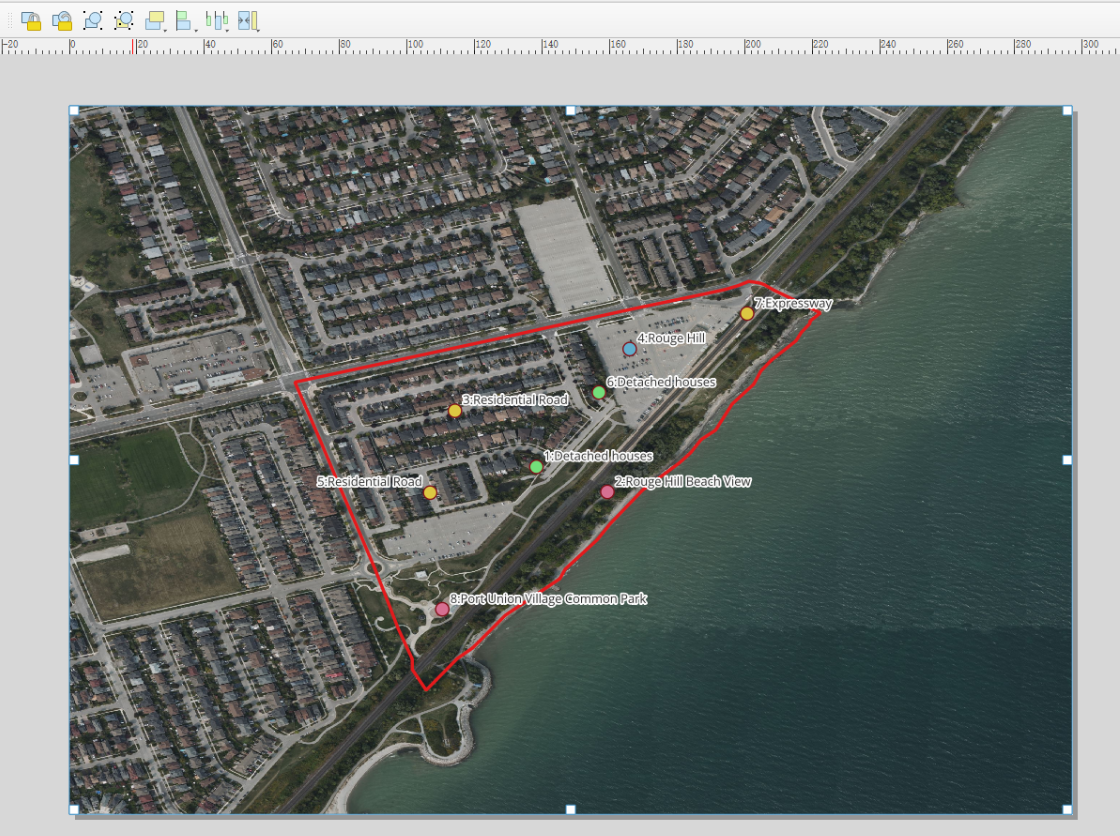
第一步选择da，创建点图层

1、选择一个包含多种证据类型、且边界相对清晰的 DA，证据类型包括：住宅密度、土地利用、交通道路
核心点就是住宅建筑不均匀或均匀即可
2、选好da之后记录，他字段里面的dauid,我这里选的是35204238
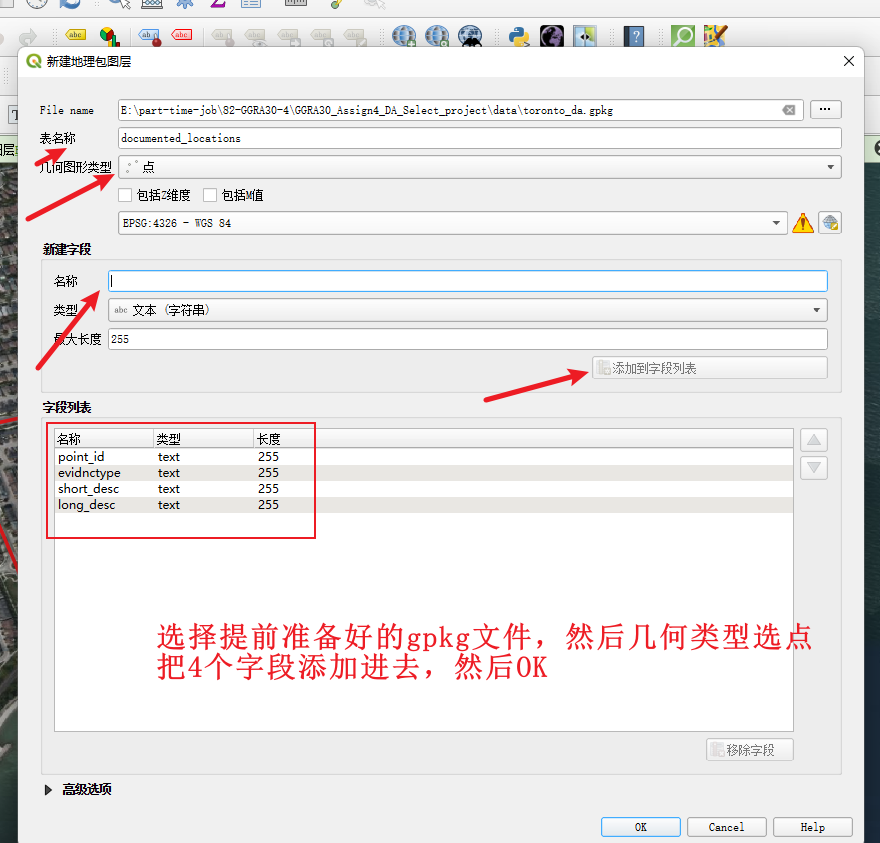
3、在预先提供的documented_locations.gpkg中创建点documented_locations图层

第二步根据你线下的拍摄创建点，编辑对应的属性

4、创建好了之后，直接就是左键选择这个图层，然后点击铅笔按钮，进行证据点的创建
point_id：从1开始编号
evidnctype：H 或 L 或 T 或 O；对应的意思分别是住宅类型证据、土地使用证据、交通/出行证据、其他证据
short_desc：短描述标签	，这里可以用地名
long_desc：长描述标签    ，这里自己看到什么就描述什么即可，可以多写点


5、你可以弄8-12个左右，每个点都要有自拍照

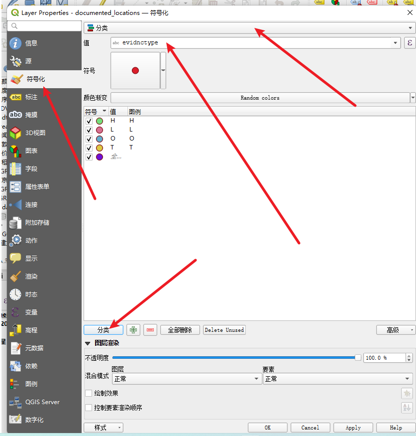
6、符号化和出图
	根据 evidnctype（H, L, T, O）进行分类着色，以便在图例中解释 
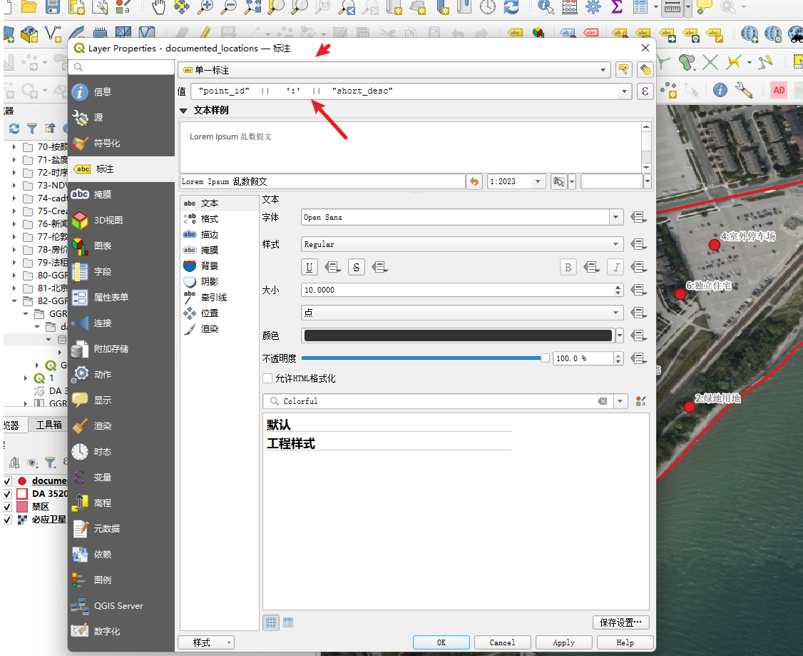
	每个地点必须用point_id 和 short_desc进行标注（例如：“1: 宽敞独立屋, 地段安静”）

第三步出图

参考工程模板

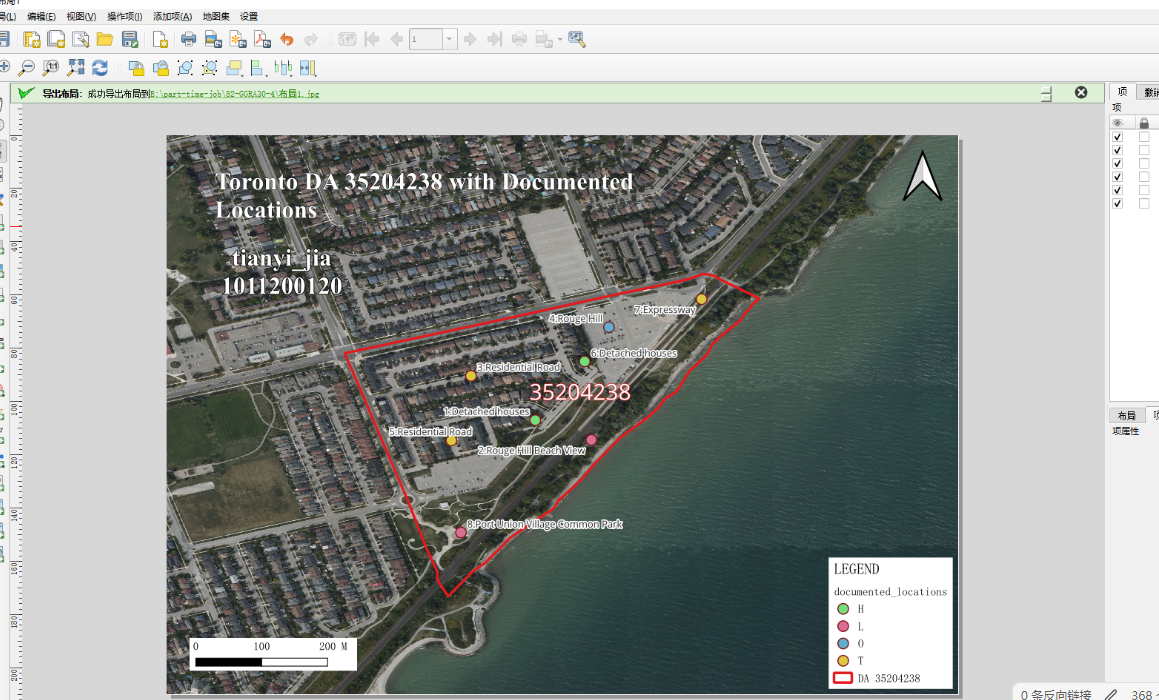
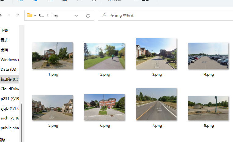
第四步拍照

照片用point_id 和 short_desc进行命名就可以了

83、GGRA30_Assign5_IntroArcGISOnline

第一步登录

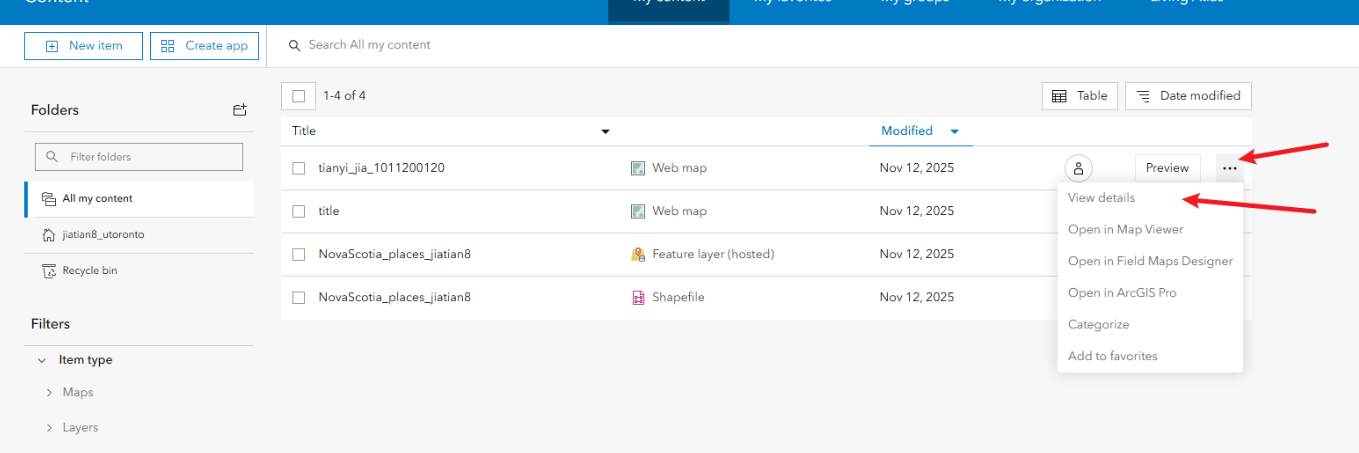
1、登录学校账号，上传证据点数据
https://utoronto.maps.arcgis.com/
上传documented_locations需要包含自己的账号UTORID：jiatian8
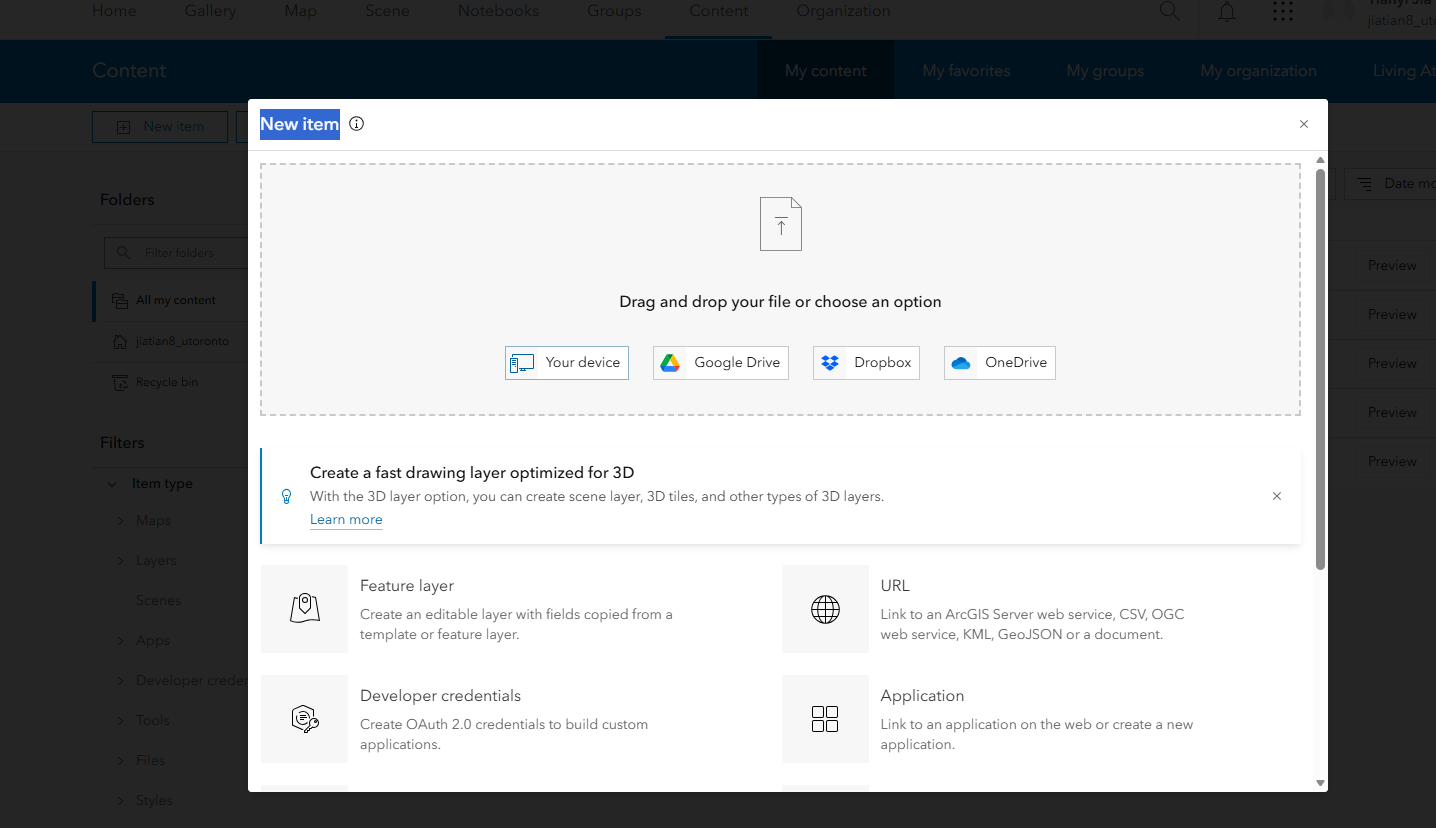
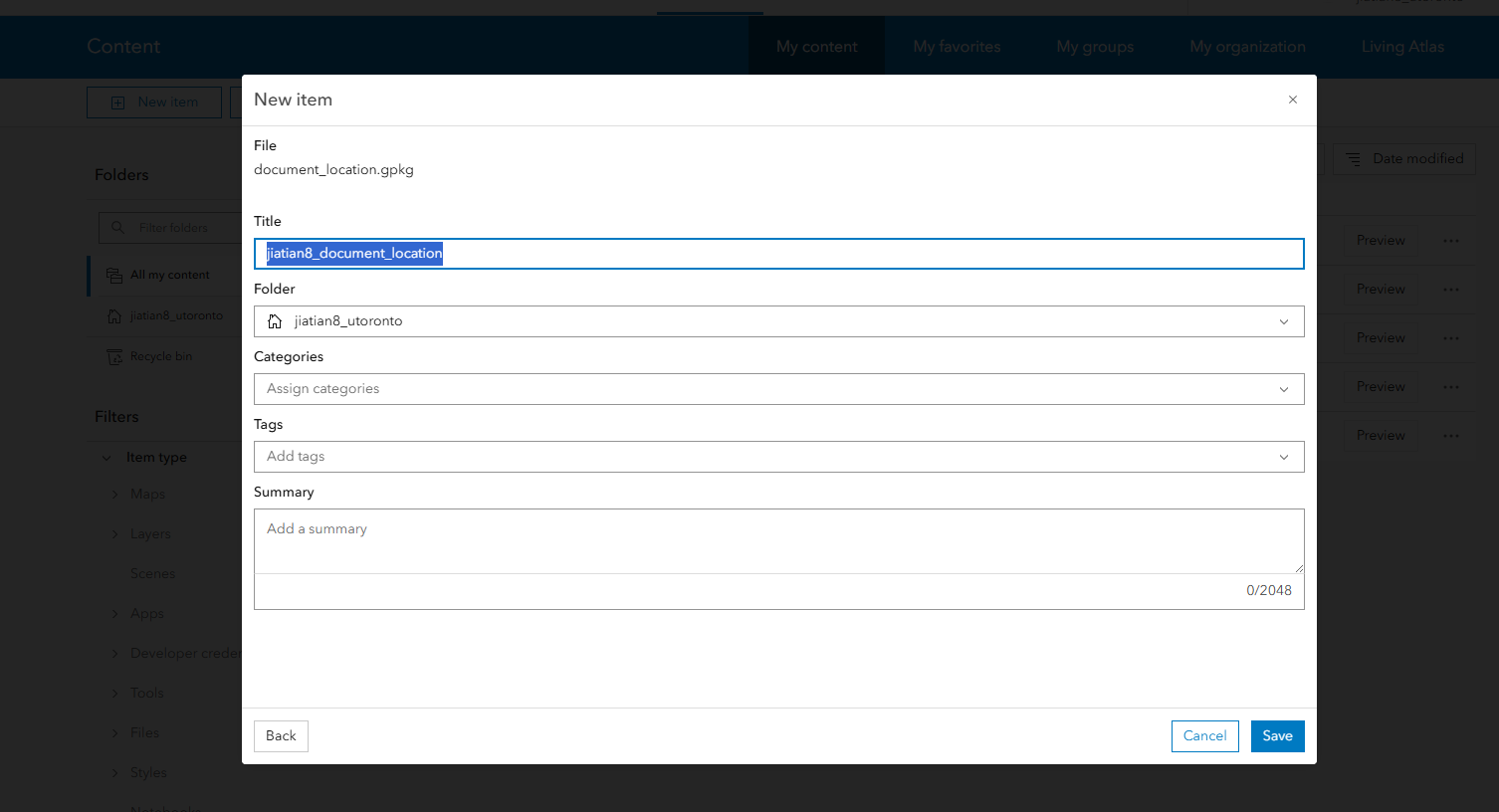
导入步骤和之前一样，通过content页面的左上角New item，就是把你得document_location.gpkg导入，命名为主要包含你的账号名就可以了jiatian8_document_location
2、上传所有的点位证据图和自拍
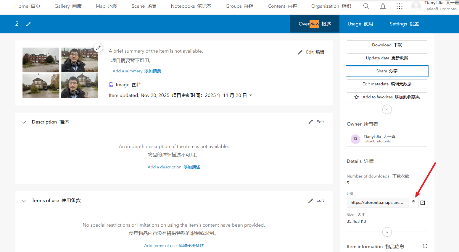
3、拿到图片的url
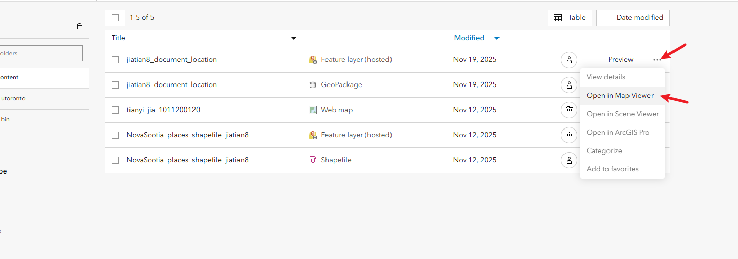
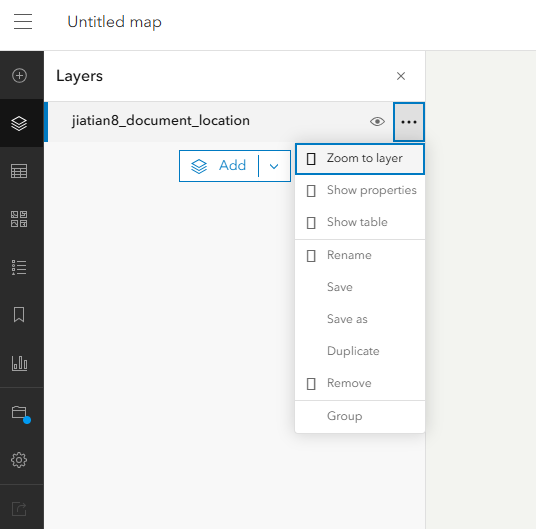
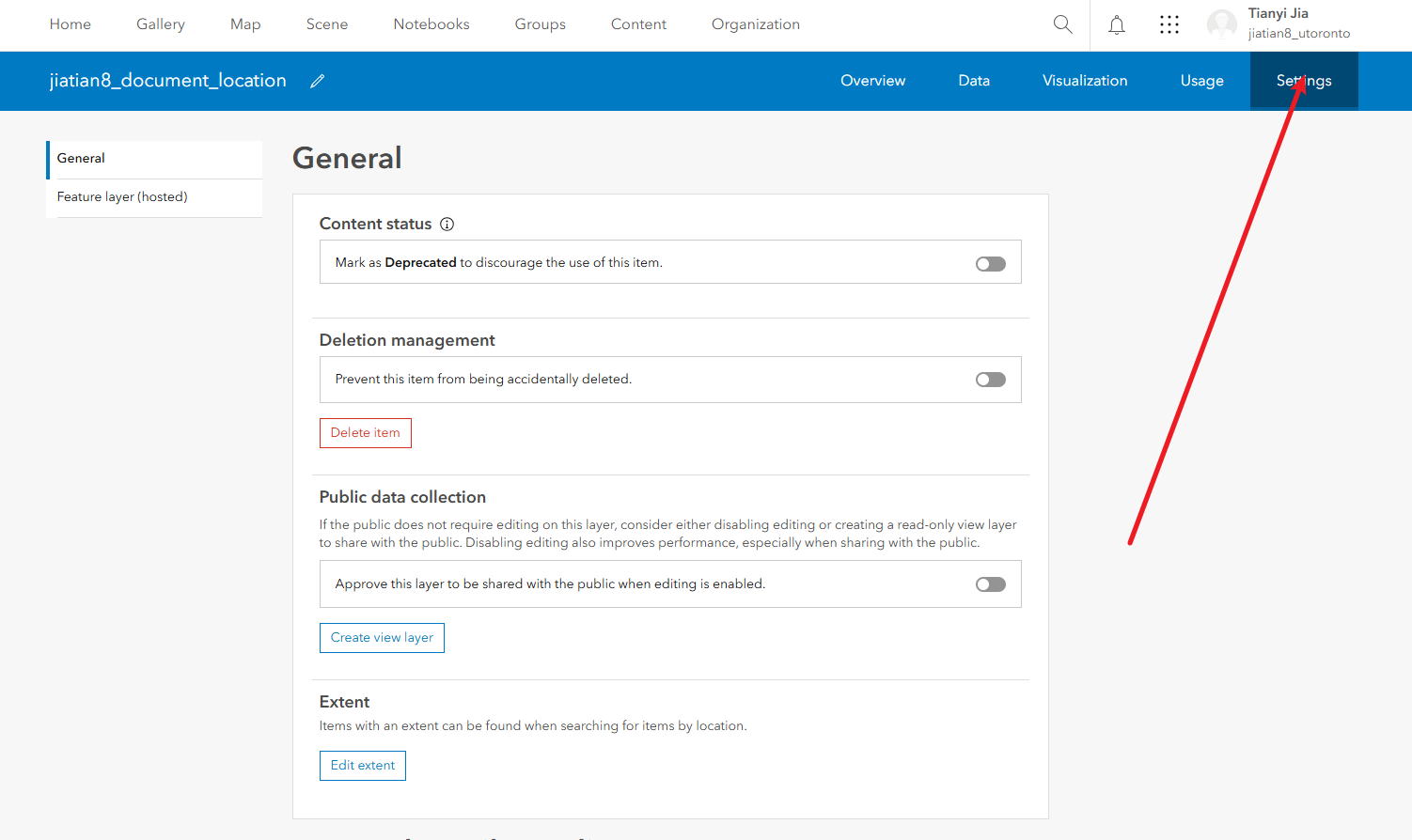
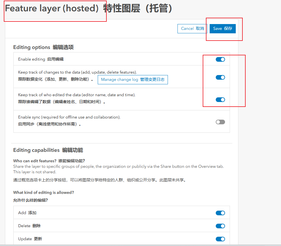
4、进入到documented_locations图层的详情页面，点击setting,往下滑，找到Feature layer，打开编辑选项卡后保存
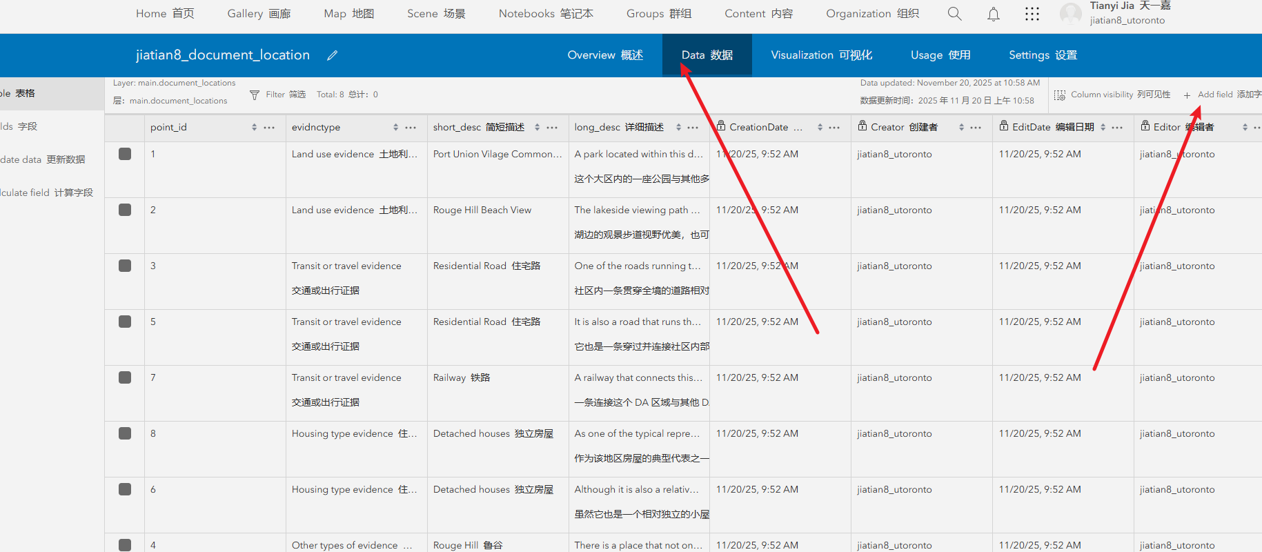
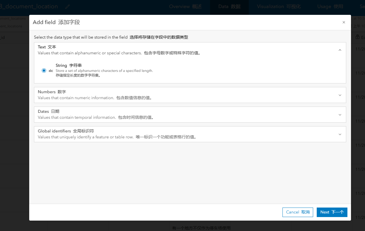
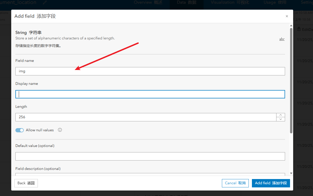
5、滑倒顶部打开data选项卡，添加字段，选择字段类型text，输入字段名，

拿到图片的url

修改图层设置让他能够修改字段

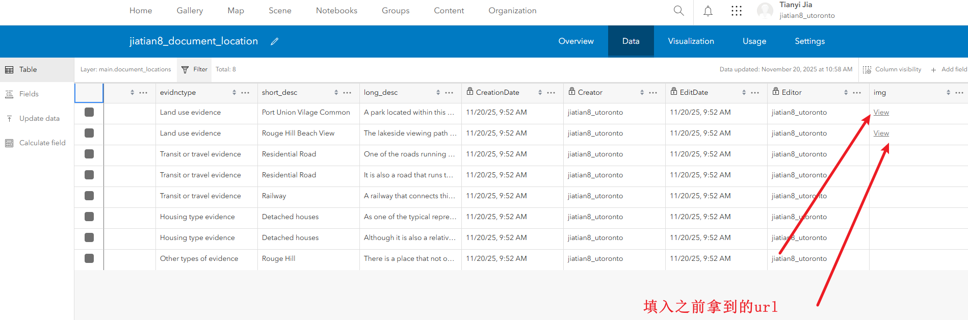
进入data添加img字段，将对应的图片url填入

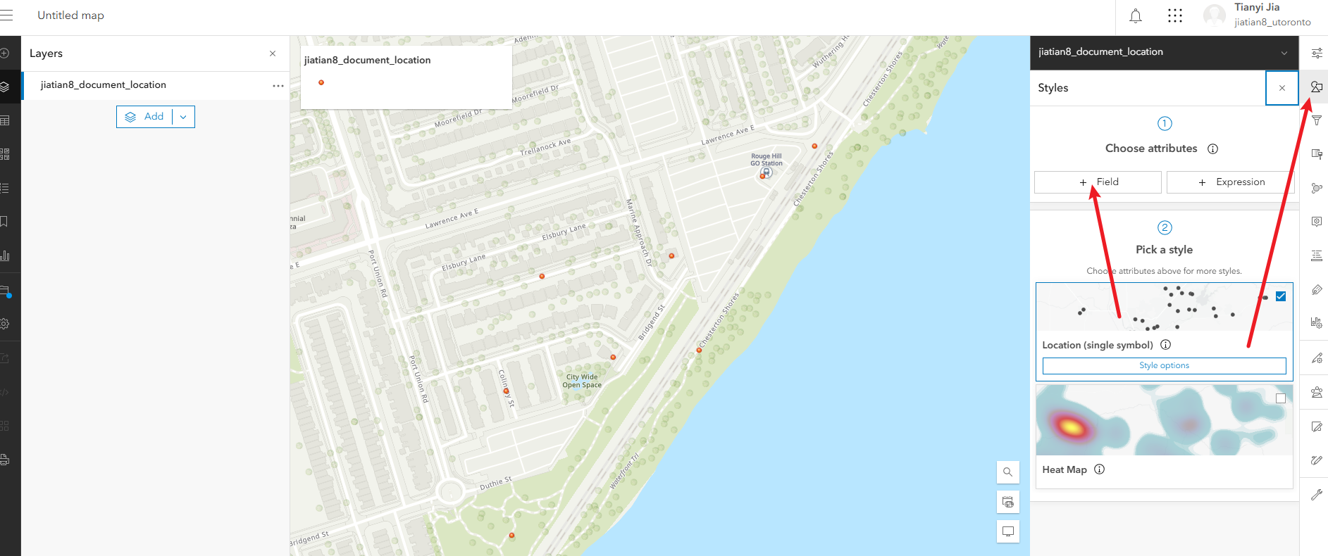
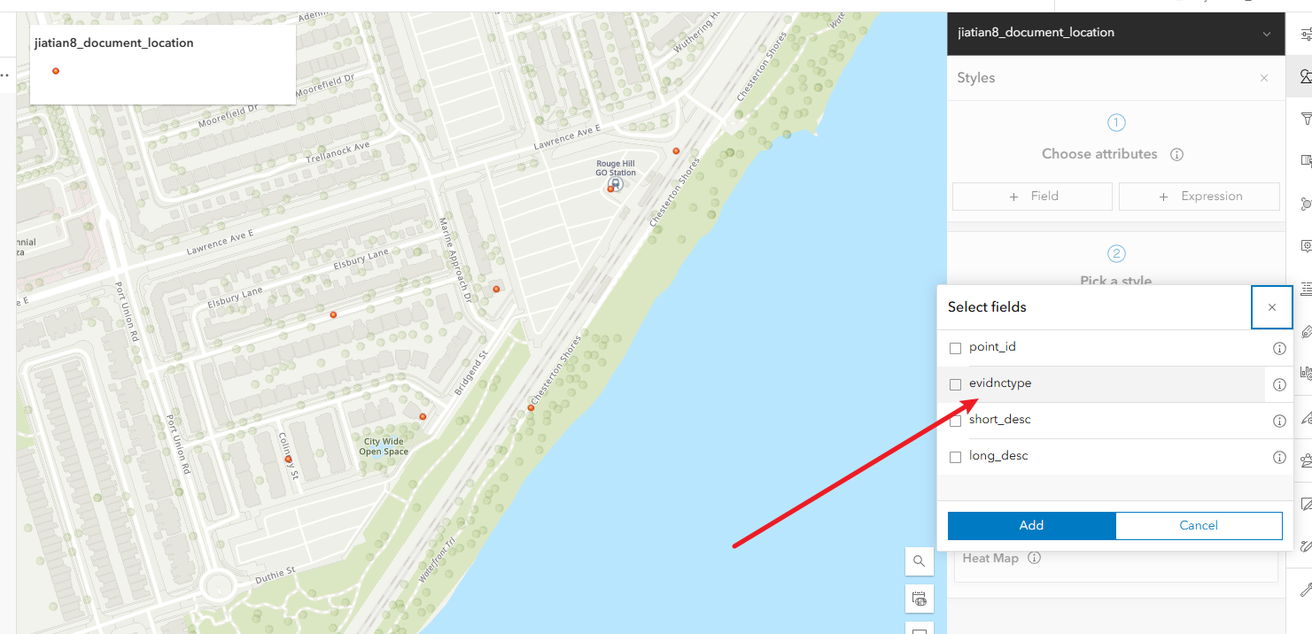
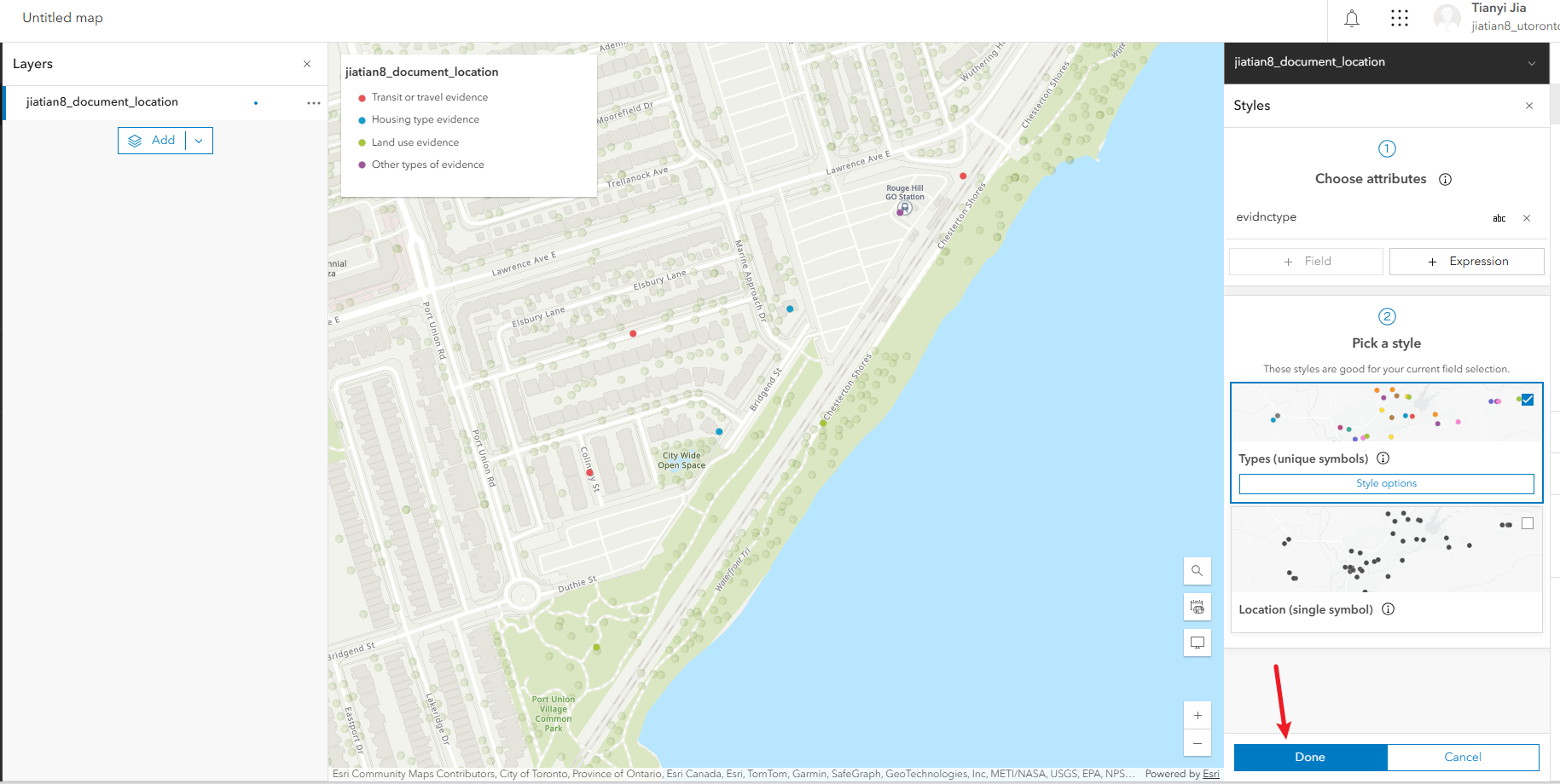
第二步配置图层

1、配置符号：右侧的style，选择field，选evidnctype，然后下方done

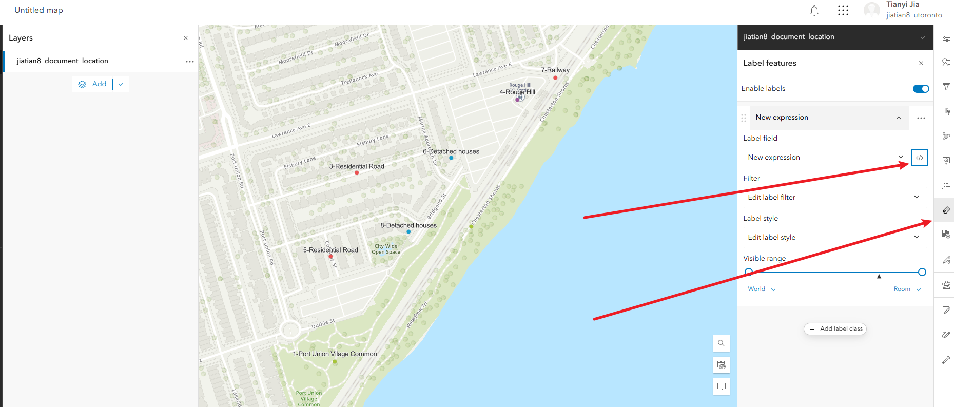
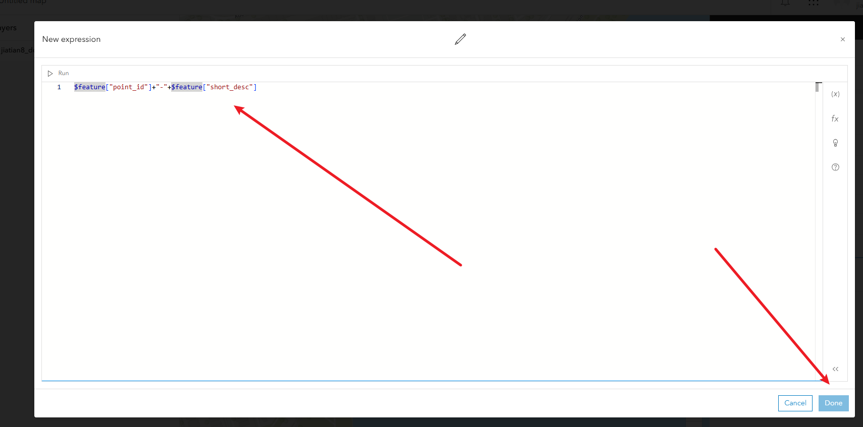
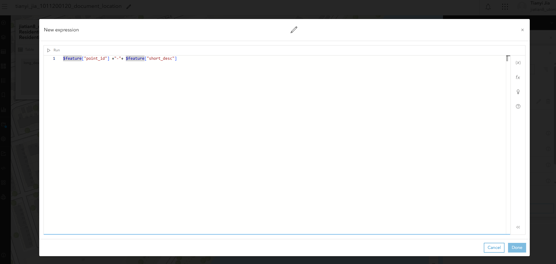
2、配置标签：右侧的lable，填入表达式$feature["point_id"]+"-"+$feature["short_desc"]

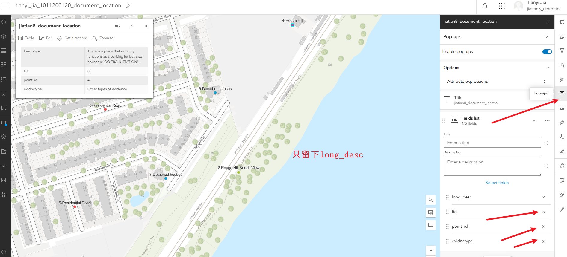
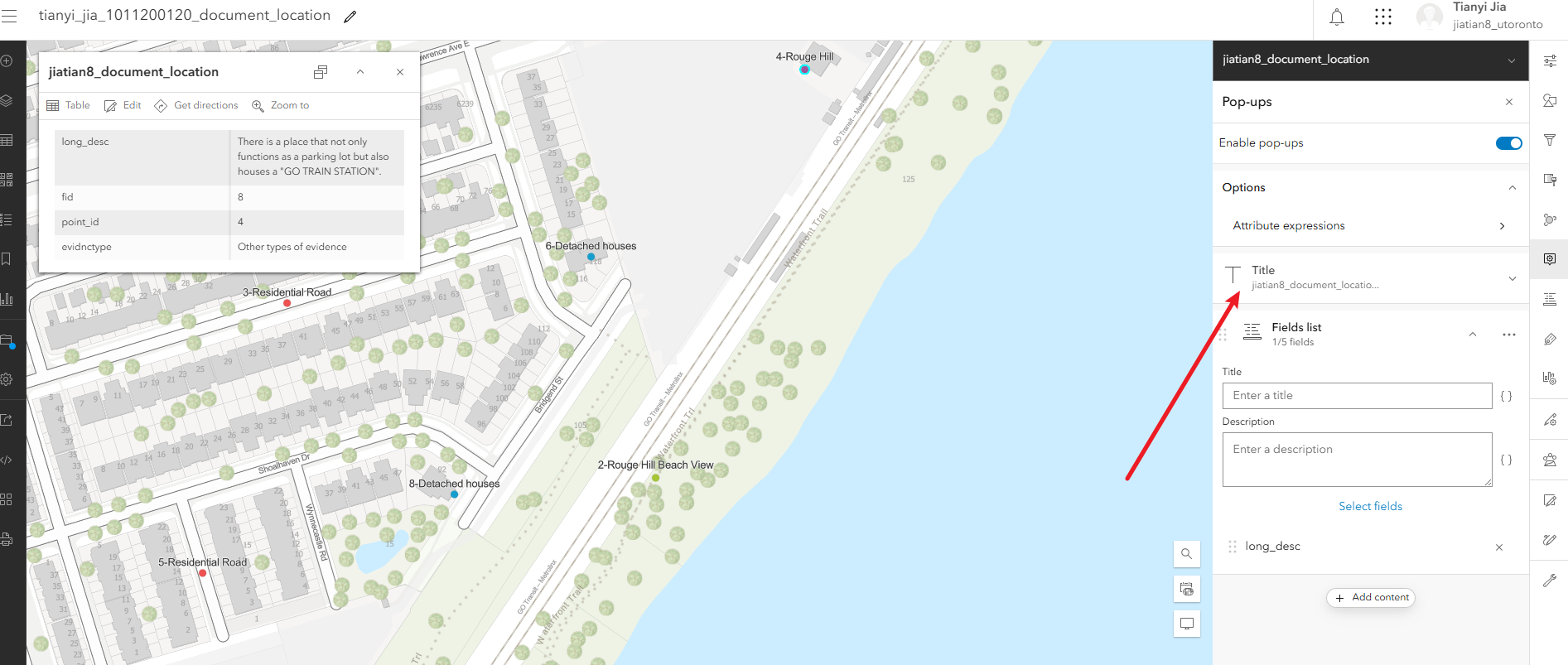
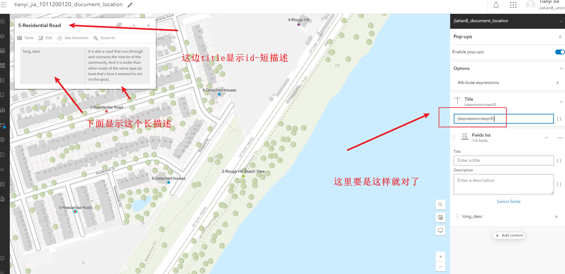
3、配置弹出属性框的显示：右侧pop-ups,把除了long_desc的字段都去掉，然后继续配置弹出的title,填入表达式$feature["point_id"] +"-"+ $feature["short_desc"]，完成后检查title下面的表达式是否为{expression/expr0}

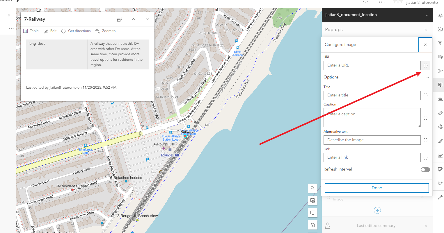
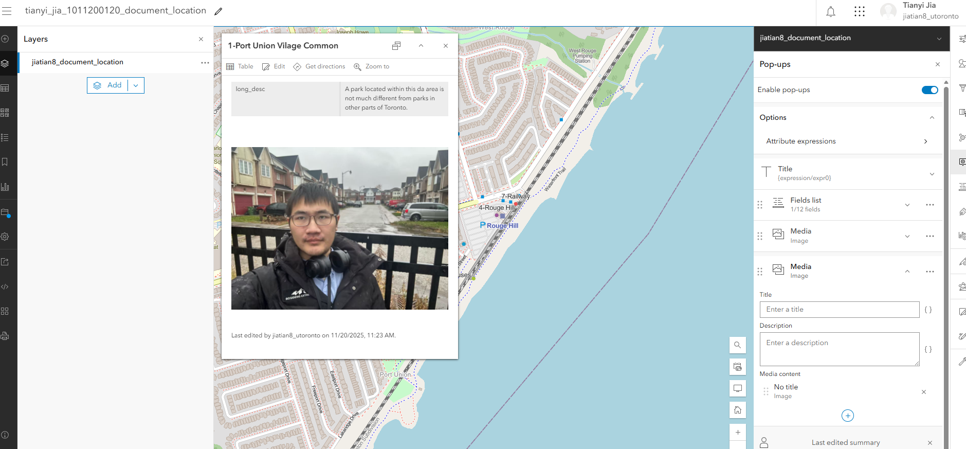
4、配置弹出面板中显示图片

配置符号

配置标签

配置属性

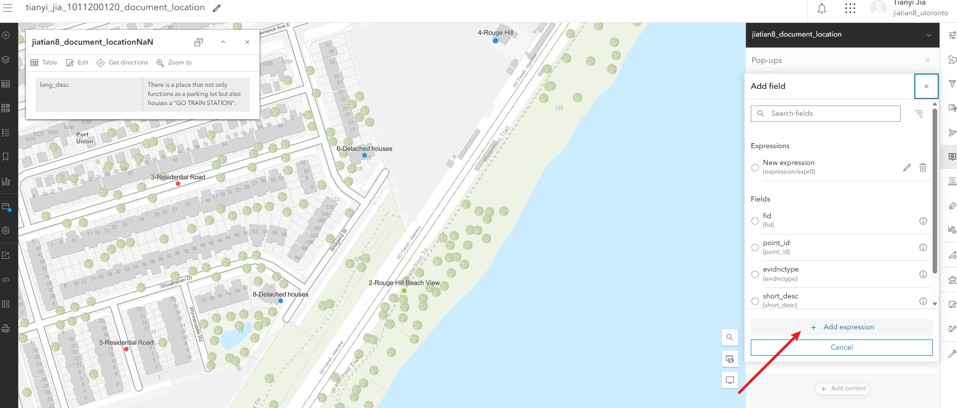
配置弹出面板中显示图片

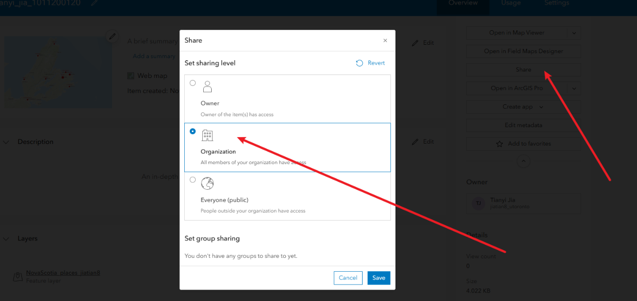
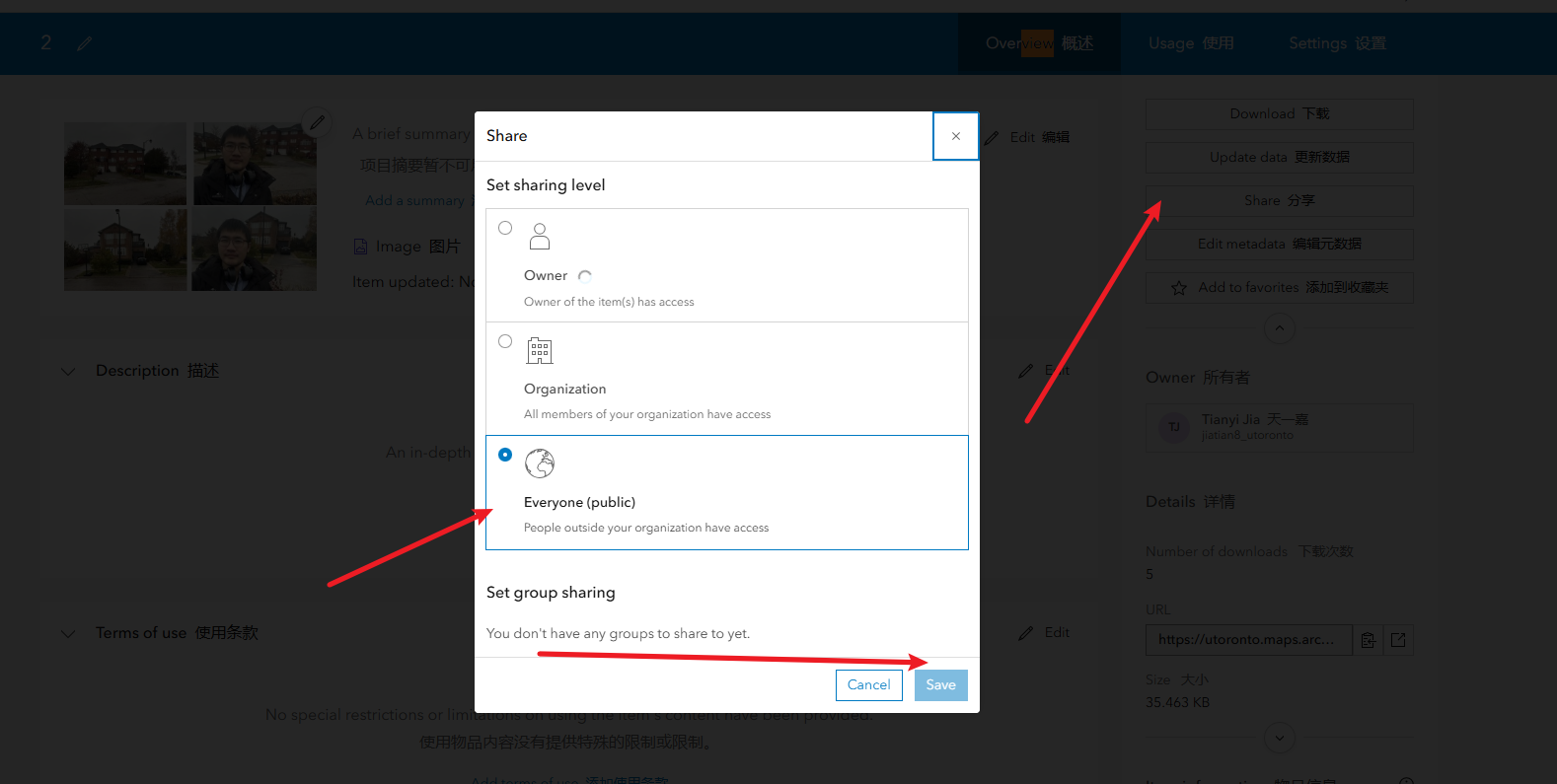
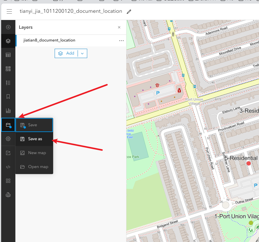
第三步保存map，设置图层共享权限，分享

1、保存map
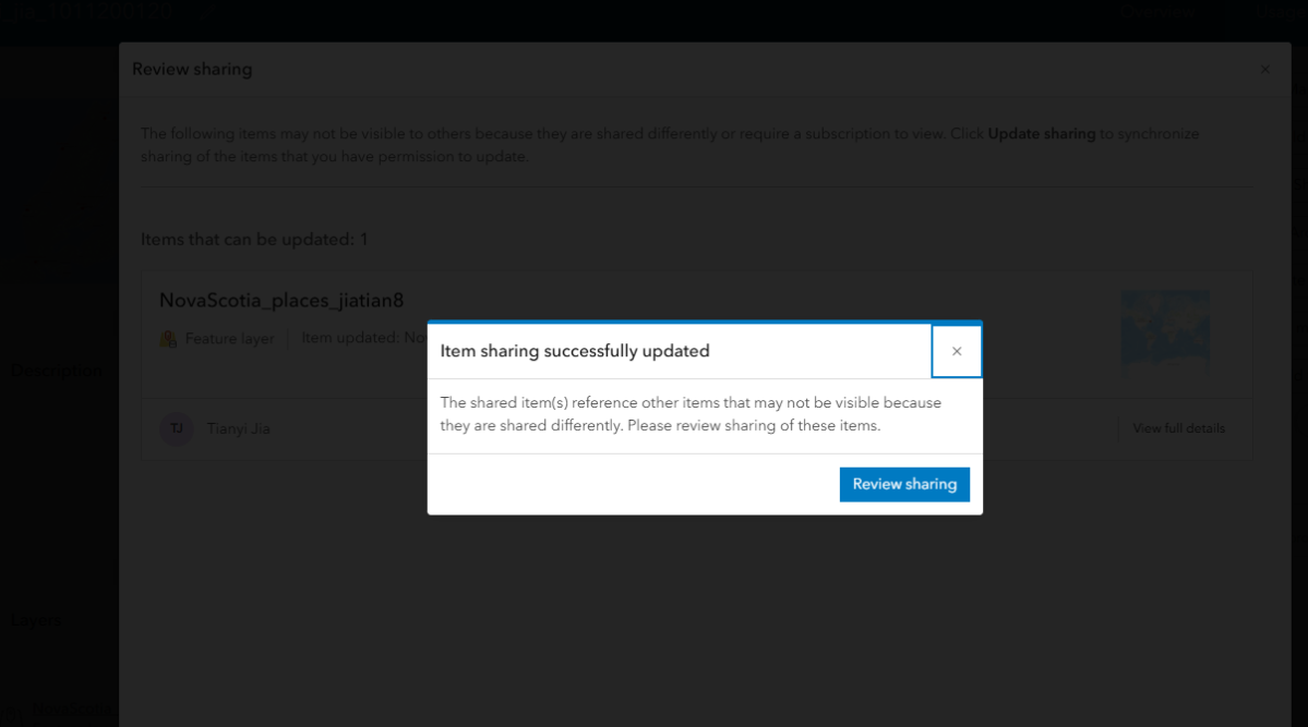
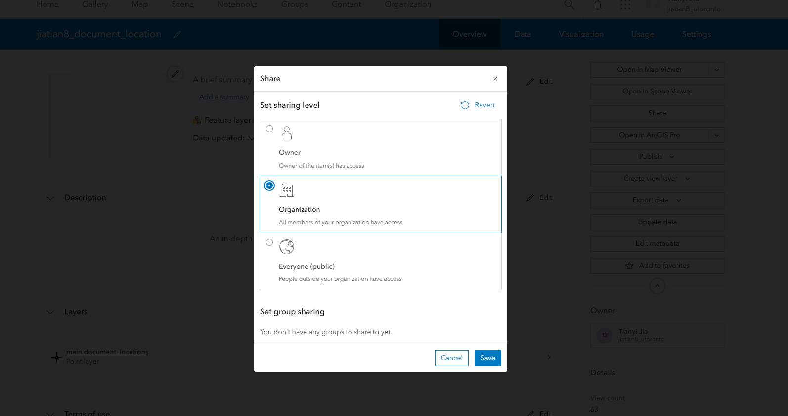
2、共享要素图层：进入您的托管要素图层 jiatian8_document_location共享Share给您的组织Organization
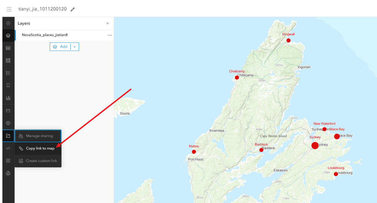
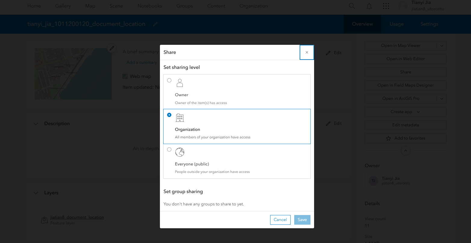
3、共享地图：一样的操作进入# tianyi_jia_1011200120_document_location
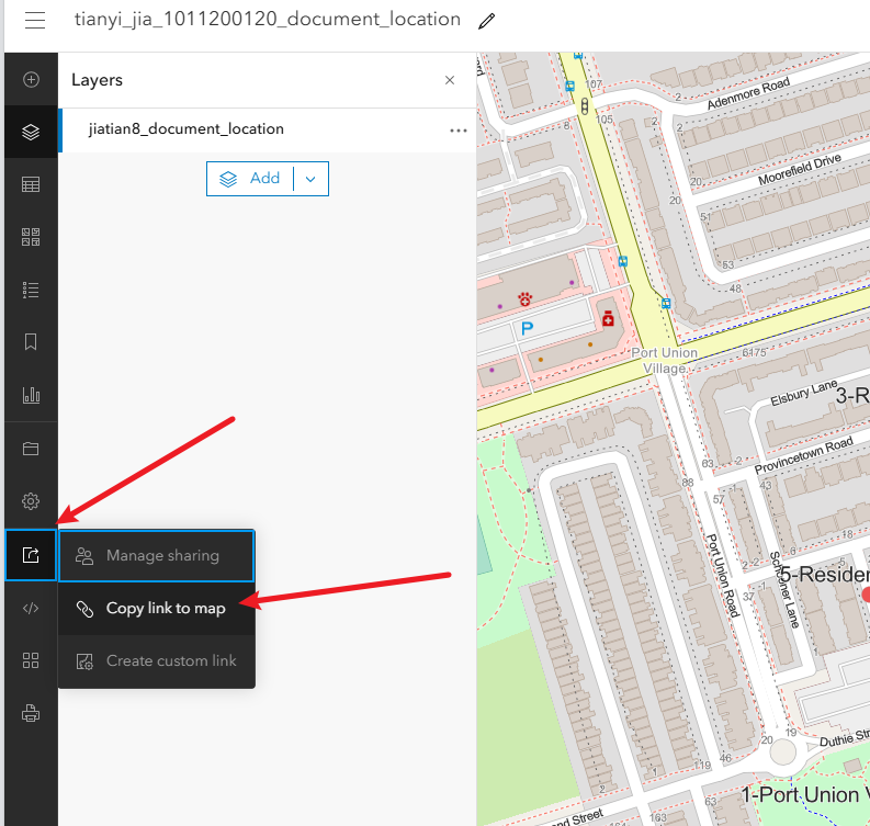
https://arcg.is/1K99KX1

共享要素

共享地图

分享地图url